

My first Kaggle challenge : the Avazu CTR contest

In October 2014, Kaggle launched a new challenge, about optimizing click-through rate prediction (CTR) based on event data provided by Avazu Inc. I embarked on a long journey for doing my best on the challenge up to its end in February 2015. I joined forces along the way with Christophe Bourguignat, and we teamed up as “The Good Timers”.
This paper will present some key insights on the challenge and the methods we used. The first part here will motivate the CTR prediction objective, and then dive into the challenge and methodology. We will publish later a second part on the algorithms we used.
We are publishing in parallel on his blog a series of articles focused on some of the more technical insights.
Motivation for CTR prediction
In 2015, $52.8 billion will be spent in digital advertising in the U.S., accounting for 30% of the overall advertising expenses. This is a 13% increase since last year, and about 5 times more than 2005. One of the keys to digital advertising’s success lies among its ability to target consumers efficiently. Using the history of queries and navigation, the publishers (Google, Bing…) can predict which ads match the most to the user and publish them accordingly.
One key predictor of interest for this task is the click-through rate probability, i.e. the probability that the user clicks on the ad.
The applications are numerous:
-
performance estimation for pricing
-
optimization of the expected gain for real-time bidding
-
variance reduction for A/B testing: when comparing two publishing policies, using powerful predictive models allows to get rid of the context as much as possible, resulting in higher test significance (just like in the Higgs Kaggle contest).
The Avazu CTR prediction contest
The provided data are structured, formatted events, with several variables, all categorical:
-
Id
-
date and hour
-
click (yes / no as 1 / 0)
-
user features:
-
device Id (several millions categories)
-
device IP (several millions categories)
-
connection type
-
device type
-
-
context features:
-
Id of visited App/Website
-
category of visited App/Website
-
connection domain of visited App/Website
-
Banner position
-
-
anonymized categorical features (C1, C14-C21):
-
9 anonymized categorical variables. Probably related to the ad+user match, past history, fatigue …
-
The metric is the usual negative log-likelihood of the model:
This metric is designed to penalize the realization of surprising events, and has some nice properties such as being lower bounded by the conditional entropy
.
The method
A Kaggle contest is not a real life problem because there is much more emphasis and feedback on performance. In real life, you can at best benchmark your performance with a legacy method or an industry standard, and sometimes get feedback from real operations.
On the other hand, in a Kaggle challenge, your score and rank are visible on the public leaderboard, and hundreds of teams are trying to climb the ladder. This is a very strong incentive to improve and test many different setups by iteration. Throughout a Kaggle challenge, we experience the « science » in « data science »: understand, experiment, interpret results, understand better and then design new experiments, and looping on again.
For this reason, we made sure we could efficiently try many algorithms and parameters and record the results. At the end, we have submitted 105 different results to the Kaggle web site, and we probably tested around 500 different models of so.
Running
In the correct mix of high tech and low tech, all the experimentations were run from the command line, with reproducible scripts. All parameters were passed on the command line (as opposed to modifying scripts) and all the data preparation was automated. The recipes for data preparation, training models, testing them and generating test files, cross-validation, and final Kaggle-ready files were written in a series of Makefile’s, and all configurations are uniquely named.
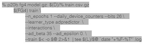
Here, we can generate a Kaggle-ready file from the command line with a « make total3.p20b.kaggle.gz”: it performs file transformation, model training, prediction, all automatically. We have thus been able to test many configurations overnight, and get the results in the morning.
An important aspect of experimenting is to record scrupulously the results of experiment along with the parameters: I did this simply on a paper notebook – low-tech and effective!
Finally, you must make sure that you are able to regenerate the result of any experiment, at any time, even if you have modified your code. Our hand-written Python code thus went from 300 to 1200 lines of Python without breaking backward compatibility. We made the new features available via command line options, keeping our former code as the command line default.
Validating and calibrating
Ultimately, you want to make sure that you estimate properly the competition metric before submitting to Kaggle, to make sure you really understand the challenge objective and avoid too frequent submissions.
We first tried to validate with a random sample taken from the dataset – it did not work. There are daily trends in the data, and training with fresh data from the same day yields better performance than for a different day. Although you can do so in real life CTR configurations, such training is not relevant for this challenge since the train and test correspond to different days.
Therefore, we trained on all training days minus the last one, tested on the last one, tuned the model by iterating, and when ready to submit, trained again on all training days and predicted on the test days. All this was automated in the Makefile.
Another important technique is to calibrate the results. Since we wanted to predict probabilities and not just a score between 0 and 1, we expect consistent results:
-
The predictions histograms should be centered on 0.17 (the fraction of ads clicked on), with a spread down to about and up to about .
-
Among N samples with prediction close enough to, say, 0.1, we should have 0.1N about positive samples.
Otherwise, the predictions must be adjusted, and it has been experimentally proven that you can improve your logloss score by calibrating.
In practice, logistic regressions are well calibrated, but other algorithms (e.g. tree-based) do improve with calibration. Thus we used calibration only as a sanity check, to verify we were not overshooting the optimal solution (which sometimes happened).
Big data, small PC
The dataset from Avazu is a sample from ten days, totaling 40M events, something you can just fit in memory if you have 16GB of RAM. Not big data, not really small either. Do you need a Hadoop cluster, or a super-computer? Or a big database server? Indeed no: the bulk of the work ran on a modest 2 years-old, 1000€ desktop PC, with a standard 4-cores i7 and 16GB of RAM, helped with a nice SSD disk. We then had 3 options:
-
use only out-of-core, online algorithms
-
sample from the whole dataset, and train only from a sample
-
split the dataset in several partitions, train on partitions and then ensemble.
Mostly we did 1., and online algorithms proved very powerful for this challenge, allowing an efficient and effective CPU-bound process (not i/o bound). Sampling proved to be too crude. We tried splitting and ensembling a bit, but it did not look very promising.
Conclusion (at the moment)
Having motivated the challenge and defined the setup, we are now ready to dive into the actual algorithms – feature preparation and modeling. We will do this in the next article on the topic.
