Quant Blog Le blog des Experts Data & IA

Recherche et développement

24/01/2020

Tabular data generation using Generative Adversarial Networks

Temps de lecture : 12 minutes

✍ Aurélia Nègre et Michaël Sok / Temps de lecture : 17 minutes

Generative models are an exciting area of research and have multiple applications. Indeed synthetic data could be used in replacement or complement of real data for simulation purpose, robustness improvement, or to handle privacy issues. That is why Generative Adversarial Networks (GANs), have had a huge success since their introduction in 2014 by Ian Goodfellow [1], their image generation being outstandingly realist. You can see more in our previous blog article here.

Image from the website: https://thispersondoesnotexist.com

A vast majority of the GANs literature focuses on images and every Data Scientist knows they are not the most frequent data source he might work on. Tabular data are indeed the most common data source. Structured data is the data that conforms to a data model, has a well-defined structure, follows a consistent order and can be easily accessed and used by a person or a computer program. Tabular data are structured data with clearly defined columns and rows (e.g Excel format).

Fortunately, there are some scientific papers that address the topic of tabular data generation. This literature was the starting point of our own implementation of tabular data generation.

Context

[latexpage]

As consultants, we were working on a project where a classifier was going into production, and we considered using synthetic data -that would be generated by a GAN- to improve its robustness.

NB: the customer and project context are confidential, therefore no information regarding the use case can be provided. Simply imagine a standard churn or fraud classifier, using Machine Learning or Deep Learning models.

We had a two-step approach in mind:

can we design a GAN that can generate realistic synthetic data in our specific context? If we can, the synthetic data could be used in replacement of real data to train the model, in addition to real data to improve the model robustness, or could be shared with other group entities that can not share real data
can we generate adversarial examples that would purely improve the robustness?

Interested by very recent papers on GANs on tabular data [2, 6, 7, 8, 9], a Proof Of Concept was launched for testing GANs in our context. The objective was to verify if data under high constraints and specificities could be generated while keeping the statistical properties needed for learning the original task of classification.

Thus we focused on Mottini et al. (2018) [2], whose problem was similar to ours, to try to answer our problem in around 60 person-days.

Our starting point – an academic paper

As mentioned in their article [2], Mottini et al. use Passenger Name Records (PNRs) data that contain travel and passenger information. Indeed, the authors are both academics (Inria) and corporates (from Amadeus, a major Spanish IT provider for the global travel and tourism industry). Amadeus’ issue with PNR data was the following: the data could not be kept for more than 3 months after the trip due to data ownership laws (GDPR). However, they wanted to train Machine Learning models to improve their company’s efficiency (e.g predict the next trip).

Therefore, they considered building a historic of synthetic data to train their models on. For such use case, GANs were the reference methodology. We note that in PNR, both categorical and numerical features with missing/NaN values are present, which makes the use of GANs quite challenging.

Thus, they proposed a solution based on Cramér GANs [3], categorical feature embedding (also known as entity embedding in the literature) and a Cross-Net layer backbone [10]. The dataset used for training was a real PNR dataset, while their evaluation focused on distribution matching, memorization and performance of inference models for two real business use cases: customer segmentation and passenger nationality prediction.

Though the real PNRs were not memorized, the synthetic matched them quite well and could be used for their use cases models training.

In conclusion, their use case was close to our own use case (tabular data, mixed types, sometimes missing values) and the paper being written by corporates, we considered their approach might be sufficiently pragmatic and transposable for us.

Reminders about GANs: Vanilla, WGAN, WGAN-GP

Before presenting our specific approach, let’s remind how the original GAN was defined (also known as Vanilla GAN):

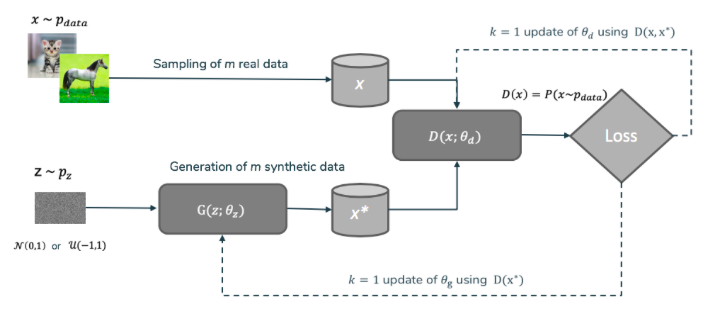
Figure 1: Vanilla GAN schema

In the above picture, two “agents” are defined: the generator G and the discriminator D. Those two names will be kept throughout this article, thus remind them well! The objective for the generator G is to deceive the discriminator into thinking its outputs are valid inputs. Symmetrically, the discriminator D should classify features into generated or real. Those opposed objectives explain where the “adversarial” part from GAN comes from.

This GAN, defined in 2014 by Ian Goodfellow et al. [1], has many extensions whether on its loss, on its network backbone or on the discriminator output. For information, the above problem from Vanilla GAN could be reformulated as a minimization problem of the Jensen-Shannon divergence. The use of Jensen-Shannon divergence posed some problems in the practical use of data generation such as:

Vanishing gradients (the gradients were way too small to learn something)
Mode collapse (a single kind of instances were generated on which the discriminator was bad at discerning if the data was fake or not)

Those problems were what motivated the use of a GAN minimizing another divergence or distance. That is how the Wasserstein GAN (or WGAN for short) was conceived, in a publication by Arjovsky et al. [4]. Many things changed between the original GAN and WGAN such as:

a new loss function was used, based on Wasserstein-1 distance
the output of D is no longer a probability of being real or not, but rather a score in the \mathbb{R} domain, which is why the discriminator is now called a critic
the optimization problem constrains the discriminator to be a k-lipschitz function, which was made possible by clipping the weights of the discriminator, or by adding a gradient penalty in its variant (known as WGAN-GP)
using an alternate optimizer than Adam (RMSProp) since the momentum in Adam posed convergence problems

The resulting GAN could be summed up in the following schema:

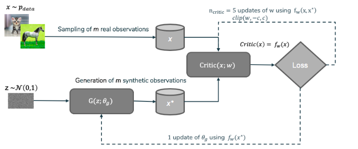
Figure 2: WGAN schema

Though we’ll not dive into the meanders of the implementation, one has to know that this implementation is optimizing an equivalent problem to a minimization of the Wasserstein-1 distance using the Kantorovich-Rubinstein duality [5] explaining the k-lipschitz constraint and the output domain.

Application to tabular data

As explained in the “Context” section, we had a classifier on which we wanted to know if it could learn on synthetic data as a first step and if generated adversarial attacks could be used for robustifying the model.

Before diving into the implementation method, let’s talk about the data specificities. Since we said that Amadeus paper restrictions were close to ours, we indeed had categorical features, as well as numerical discrete and continuous ones. We also had the obligation of not replicating the observed data points (obviously, since otherwise we would have a kind of random oversampling method). Some multimodal distributions were also mixed in. Finally, we had around 100 features with significant dependencies (such as the sum of some features is lesser than another).

The classifier was binary, thus we knew that for testing a trained model on synthetic data, we could use the label knowledge. Regarding the label, three methods could be used:

ignoring the label knowledge and generate the label as any other feature
creating two generation models, one per label
using the label as a generation input, similar to Conditional GAN (cGAN).

We chose the second method because of time constraints, though the third option is tempting because of its smallest restrictions when dealing with a multi-classification problem.

For this generation problem we tested multiple GANs implementation:

Vanilla GAN [1]
Wasserstein-GAN [4]
Wasserstein-GAN Gradient Penalty [4]
Cramér GAN [3], with and without crossnet layers
Tabular GAN [7] (on-shelves implementation, see https://github.com/DAI-Lab/TGAN)

The POC objective was twofold: testing GANs in our specific problem and implementing a generation pipeline and performance criteria. We’ll introduce how we choose to implement our generation pipeline:

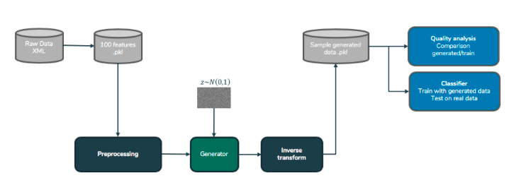
Figure 3: Generation and performances pipeline

As shown in the above figure, raw data (in XML format) is transformed into classifier features (in pickle format) which we’ll preprocess into a GAN input. After training, the generator creates new observations already preprocessed which we’ll pass into an inverse transformer. This will transform the new observations into the original features domain, and those will be saved into a pickle format. And those generated features will be subject to quality analysis tests as well as “model-compatibility” tests, which we’ll define later on.

As seen above, the generation is model-specific and the features created may have sense only for our specific use-case, which was acceptable in our case. However, if you can, try to generate data as raw as possible for increasing model-compatibility tests.

The preprocessing part defined is a transformer (that can inverse-transform) of the data from an original feature domain into a neural network acceptable domain. Mainly scaling is done, but for very skewed distributions, you may be tempted to cut the distributions’ outliers. That’s why in our case we had quantile 99.9% maxing distributions for cutting very long queues in the distribution. We also made a PCA, since our generation model was quite slow to fit, we chose to decrease as much as possible our dimensions to accelerate the process. Furthermore, generating the principal components instead of “raw” features was obviously providing better row-dependencies between our generated columns.

The generation pipeline being defined, we’ll now define the different parts of our generation model.

The Cramér GAN architecture

As introduced before, we used a specific kind of GAN named Cramér GAN proposed by Bellemare et Al., from Google Deepmind team. On contrary to the WGAN, this one tries to minimize the energy distance. This distance can be defined as follow:

D(u, v) = \left(2 \mathbb{E}\left[X - Y\right] - \mathbb{E}\left[X - X'\right]-\mathbb{E}\left[Y - Y'\right]\right)^{\frac{1}{2}}

where X and X’ (resp. Y and Y’) follow the same distribution u (resp. v).

We chose this distance mainly because of one of its property, the “unbiased sample gradients”. It means that when computing the gradients on a sample, it is equal to the true loss gradient. However even now, this is debated in the literature.

As a side note, since the Energy GAN name was already taken, they had to take another. Cramér distance is equivalent to the energy distance in the univariate case modulo a coefficient.

This GAN is very similar in essence to the WGAN-GP, but with one difference: the need of two distinct noises to compute the loss (being associated to the energy distance, it needs two samples of the generated distribution):

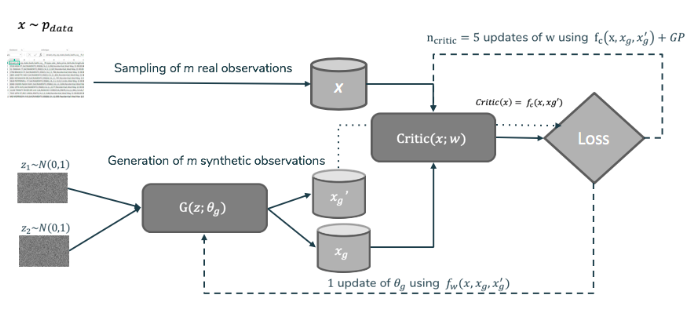
Figure 4: Cramér GAN schema

Cross-Net layers

Inspiring our implementation from the Amadeus one, we also used Cross-Net layers. Though not that known, it’s in fact really simple. The intuition behind this is to directly compute the inputs interaction terms with a cartesian product. Those will then feed a matrix product with a weight vector. This output will then be added with a bias and the original input. It was originally proposed by Wang et al. [10] from Stanford and Google.

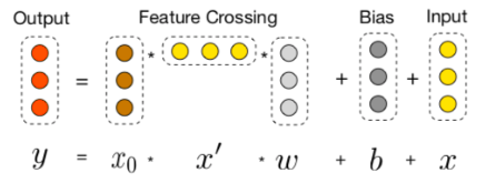
Figure 5: Cross-Net layer schema

When we have lots of interactions, this implementation becomes interesting because of its native way of handling interactions. Beware however of the increase of computation time, especially in high dimension problems.

Our GAN backbone

After defining our different specific elements in the GAN networks, the final GAN backbone can be summed up by the following schema:

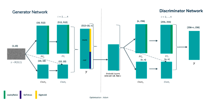
Figure 6: Our GAN Architecture

For the generator, the input noise is split between a first neural network fully connected with LeakyReLU activation, 4 layers and 512 nodes in each and a second neural network with 4 cross-net layers. Those two networks are then concatenated and aggregated into a dense layer with sigmoid activations for continuous features and softmax activations for categorical features.

The discriminator takes the input as such for continuous features but uses Entity Embedding for categorical features (basically a linear dense layer without bias from categorical one-hot encoding). This new representation is now passed a similar network with 5 fully connected layers and 4 cross-net layers concatenated before passing a linear dense layer of wanted dimension. The final dimension is indeed parameterisable since energy distance is a multivariate distance.

The optimisation was done with classical Adam optimizer.

On a side note, entity embedding is not mandatory if we made some preprocessing for transforming the encoding of categorical features with PCA (should be applied only if few modalities per categorical features) or with FAMD (more appropriate when handling both continuous and categorical features).

Synthetic data quality metric

For comparing methods, we decided on a set of performance metrics. Those can be split into three majors groups:

Univariate consistency metrics
- Statistical tests of same distribution (Kolmogorov-Smirnov, \chi^{2})
- Distribution distances (Wasserstein-1, Energy and Total Variation distances)
- Distribution plots for manual checking (real vs synthetic)
Global consistency metrics
- Validation of business rules such as business constraints on features
- Model compatibility – training on synthetic data and testing the model on real data
- Separability of our data ie. training a discriminator on generated and real data and check if it can split well the dataset between the two sources of data. It’s basically the same objective as the optimal discriminator in the original GAN, which is not present as such in Cramér GAN.
Diversity metrics
- Distance to the closest neighbor with euclidean distance in a scaled representation
- Number of features different than those of the closest neighbor

The plots are a good way to see manually if a GAN is generating wrong distributions on specific features. For instance, the following distributions were relatively well captured:

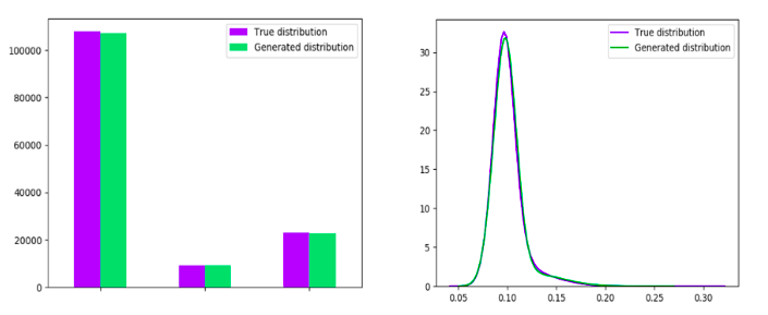
Figure 7: Distributions well-captured

Most features were accurately generated. Unfortunately, some features have some peculiarities such as multiple modes. Especially in our case, we did have problems generating such features as shown in the following plots:

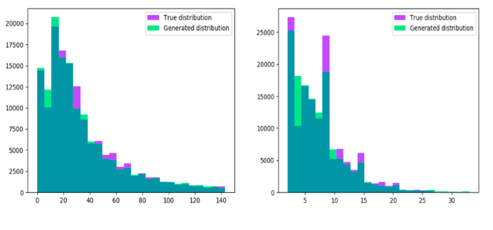
Figure 8: Multimodal distributions with some problems in generation

As you can see, the GAN tends to smooth the generation between two modes, creating a discrepancy with the actual distribution.

Final results

The results are shown in the following table:

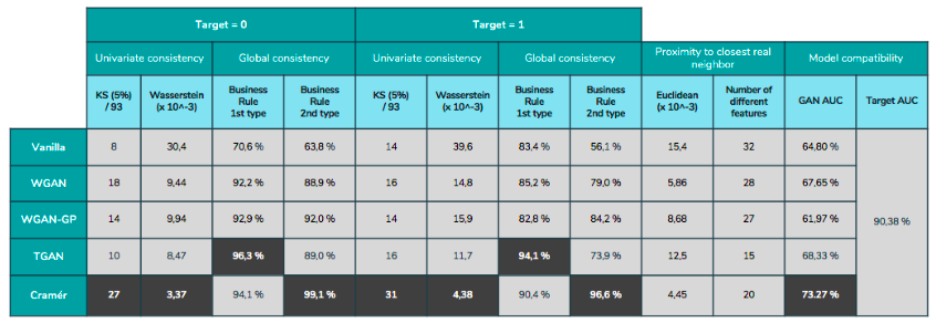
As you can see, the Cramér GAN seems to dominate the benchmark with the best results in nearly all the metrics. One kind of the business rules seems to be better captured by the TGAN, though Cramér GAN still offers good results. The proximity is not highlighted in this case since we cannot really judge if a proximity is better than another. We can just verify if an observation is close to its nearest neighbour.

One metric is not present in this specific table: separability. Depending on the strength of the separator we could go from 70% of separability (with 50% being the theoretical best score) and 90% with a very good separator.

Unfortunately, we couldn’t reach the best AUC with model-compatibility in our use case with a loss of 15 points which is way too much for production. However, the fact that we could attain up to 73% is quite good, knowing that we only had around 60 person-days for this POC. It was quite interesting to see a GAN application with real data which have specificities (long tails, multimodal distributions..) not always present in research datasets.

Small tips for those who want to tests Vanilla GAN, beware of the mode collapse which can be easily reached (in our case without some kind of regularizer, the GAN learnt one specific kind of observation after… one epoch).

Conclusion

We managed to define a pipeline for generating data as well as checking with some kind of performance metrics. We managed a relatively good separability with respect to other publications (best seen was around 70%). Finally, the model-compatibility, though still insufficient, could be seen as a good start for further researches!

However, such good results come with constraints such as time: the final model trained for 3 days which is quite long for creating a generator and calibrating it. Also, during the mission, we found this part of the GAN literature not mature yet. As an example, there is no clear research on why a specific noise should be applied as input of the generator.

Like many other tasks, but especially on this one, massive feature engineering was done in order to have a qualitative generation (be sure on the data type of the output, a discriminator can be performant if the generation and the real dataset are encoded on different types such as float32 and float64).

Next steps

As a next step, we found the idea of integrating the model-compatibility loss into the generation loss interesting. Though the generator becomes use-case specific, it’s a possibility to explore in order to increase our scores.

We also want to know the effects of noises inputs on generation. Since our use-cases deal with discrete data, a discrete noise (in complement to a gaussian or uniform noise) could be implemented in order to match the latent space with the target domain.

References

[4] Arjovsky, M., Chintala, S., & Bottou, L. Wasserstein GAN, 2017.
[5] L.V. Kantorovich, G. Rubinstein. On a space of completely additive functions, 1958.
[10] Wang, R., Fu, B., Fu, G., & Wang, M. Deep & Cross Network for Ad Click Predictions, 2017.