

Time Series Feature Extraction

Time Series Feature Extraction: An Overview of Open-Source Packages
Introduction
Time series data is a type of data that is collected over time, often at regular intervals. Examples include stock prices, weather patterns, and sensor readings. Analyzing time series data can be challenging due to its high dimensionality and complexity. One approach to simplify the analysis is to extract meaningful features from the data, allowing to describe its temporal structure. In this article, we’ll provide an overview of time series feature extraction and highlight some of the most popular open-source packages available for this purpose.
Types of Time Series Features
There are several types of features that can be extracted from time series data. Some common types include:
- Statistical Features: These features describe the distribution of the data over time, such as mean, standard deviation, and skewness.
- Frequency-Based Features: These features describe the frequency content of the data, such as Fourier coefficients and spectral entropy.
- Wavelet-Based Features: These features describe the time-frequency characteristics of the data across different scales, including wavelet coefficients and wavelet entropy.
The extraction can be applied on the whole data set or on a window. Extracting the features globally or on specific windows depends on the use case and the problem. The features extraction packages do both, so, you have to pay attention during the feature selection part.
Open-Source Packages for Time Series Feature Extraction
On python, there are several open-source packages available for time series feature extraction. Here are some of the most popular ones:
Tsfresh
This python package is designed to make it easy for users to extract a large number of features from time series data, which can then be used for machine learning tasks such as classification, regression, and clustering.
The package contains over 1200 time series features, including various statistics (mean, standard deviation, skewness, etc.), autocorrelation, and time series complexity measures. tsfresh can extract features from both univariate and multivariate time series data and can handle missing values and irregular time series data.
One of the key features of tsfresh is its ability to automatically calculate many time series features using a variety of techniques. These techniques include rolling window functions, aggregation functions, and fast Fourier transform (FFT). The package also offers feature selection methods, such as variance thresholding and correlation-based feature selection, to help users choose the most important features for their specific task.
tsfresh is designed to be easy to use and integrate with other Python packages. It offers efficient parallel processing capabilities, which can be used to speed up feature extraction on large datasets. tsfresh also includes built-in functionality for handling time series data in various formats, such as pandas DataFrames and numpy arrays.
Overall, tsfresh is a powerful tool for time series feature extraction and analysis. Its extensive library of features and efficient processing capabilities make it an excellent choice for a wide range of time series tasks.
Here are some examples of feature extraction techniques:
- Statistical features: Statistical features are measures of the distribution of the time series data. Some of the most commonly used statistical features implemented in tsfresh include mean, median, standard deviation, skewness, and kurtosis.
- Autocorrelation features: Autocorrelation features are measures of the similarity between a time series and a shifted version of itself. Some of the most used autocorrelation features in tsfresh include autocorrelation coefficients and partial autocorrelation coefficients.
- Time series complexity features: Time series complexity features are measures of the complexity or irregularity of a time series like Hurst exponent, Lyapunov exponent, and sample entropy.
Here is an example of using Tsfresh in real case:
Import libraries:
import pandas as pd
import numpy as np

import seaborn as sns
import matplotlib.pyplot as plt

from sklearn.model_selection import train_test_split
from sklearn.ensemble import RandomForestClassifier

from sklearn.model_selection import RandomizedSearchCV, GridSearchCV
from sklearn.metrics import confusion_matrix,classification_report

from sklearn import metrics

from xgboost import XGBClassifier
Read Data: we read 2 data frames which respectively represent the number of Amazon’s and Apple’s tweets. We plot the first 100 records of each.
apple_path = "https://raw.githubusercontent.com/numenta/NAB/master/data/realTweets/Twitter_volume_AAPL.csv"
amazon_path = "https://raw.githubusercontent.com/numenta/NAB/master/data/realTweets/Twitter_volume_AMZN.csv"

df_appl = pd.read_csv(apple_path, sep=",", on_bad_lines='skip')
df_amzn = pd.read_csv(amazon_path, sep=",", on_bad_lines='skip')

# Create a figure and axis object
fig, ax = plt.subplots()

# Plot the time series
ax.plot(df_appl.iloc[:100].index, df_appl["value"].iloc[:100])

# Set labels and title
ax.set_xlabel("Date")
ax.set_ylabel("Value")
ax.set_title("My Time Series Plot")

# Display the plot
plt.show()
fig, ax = plt.subplots()

# Plot the time series
ax.plot(df_amzn.iloc[:100].index, df_amzn["value"].iloc[:100])

# Set labels and title
ax.set_xlabel("Date")
ax.set_ylabel("Value")
ax.set_title("My Time Series Plot")

# Display the plot
plt.show()
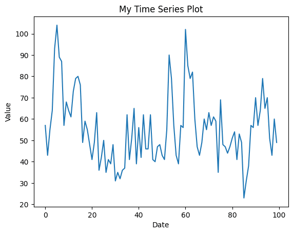
Figure 1: The number of Apple’s tweets
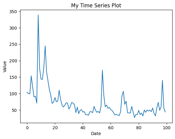
Figure 2: The number of Amazon’s tweets
Features extraction (Tsfresh): in this part, we will split the data into slices each containing 200 records. totally, in each dataframe we have 79 slots. We will try to extract features from time series using Tsfresh. More precisely from each solt of a given time series, Tsfresh will extract the features exhaustively using the « extract_features » function which takes the dataframe as input, column_id: column contains the number of each slot, column_sort: column used to sort the data usually it’s the timestamps.
def extract_features_tsfresh(df, label):
    df["slot_number"] = df.index // 200
    df["slot_number"] = df["slot_number"].astype(object)
    df_extracted_features = extract_features(df, column_id="slot_number", column_sort="timestamp")
    df_extracted_features["Time_series"] = label

    return df_extracted_features

def features_selection_tsfresh(df):
    impute(df)
    df_selected = select_features(df.drop("Time_series",axis=1), df["Time_series"])
    df_selected["Time_series"] = df["Time_series"]

    return df_selected

def preprocess_dataframes(df_0, df_1):
    df_0 = extract_features_tsfresh(df_0, 0)
    df_1 = extract_features_tsfresh(df_1, 1)

    df_concat = pd.concat([df_0, df_1], ignore_index=True)

    df_training = features_selection_tsfresh(df_concat)

    return df_training

df_training = preprocess_dataframes(df_appl, df_amzn)
df_training.shape
Select the most important features: we use tsfresh’s « select_features » function and the importance matrix to select the most explanatory variables that could help us differentiate between the two time series. We only select the first 20 variables.
X_train, X_test, y_train, y_test = train_test_split(df_training.drop("Time_series",axis=1), df_training["Time_series"], test_size=0.3, stratify=df_training["Time_series"])
clf = RandomForestClassifier()
clf.fit(X_train,y_train)

importances = clf.feature_importances_
indices = np.argsort(importances)

selected_features = list(np.array(X_train.columns)[indices[::-1][:20]])
X_train, X_test = X_train[selected_features], X_test[selected_features]

clf = RandomForestClassifier()
clf.fit(X_train,y_train)

importances = clf.feature_importances_
indices = np.argsort(importances)

fig, ax = plt.subplots(figsize=(18, 10))
ax.barh(range(len(importances)), importances[indices])
ax.set_yticks(range(len(importances)))
_ = ax.set_yticklabels(np.array(X_train.columns)[indices])
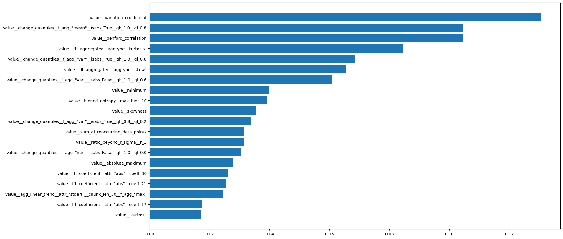
Figure 3: Features importances extracted with tsfresh
Train a Random Forest model: we will call the train_evaluate_model function to perform a cross validation training and evaluate the performance of the model.
param_grid = {'max_depth': [2,3,5,10,15,20,50], 'max_leaf_nodes': [2,5,10,15,20], 'min_samples_leaf': [2,5,10],'min_samples_split':[2,5,10,12,15],"n_estimators": [16,32,64, 128, 256,512]}
acc_rf_tsfresh = train_evaluate_model(X_train, y_train, X_test, y_test, RandomForestClassifier(), param_grid)
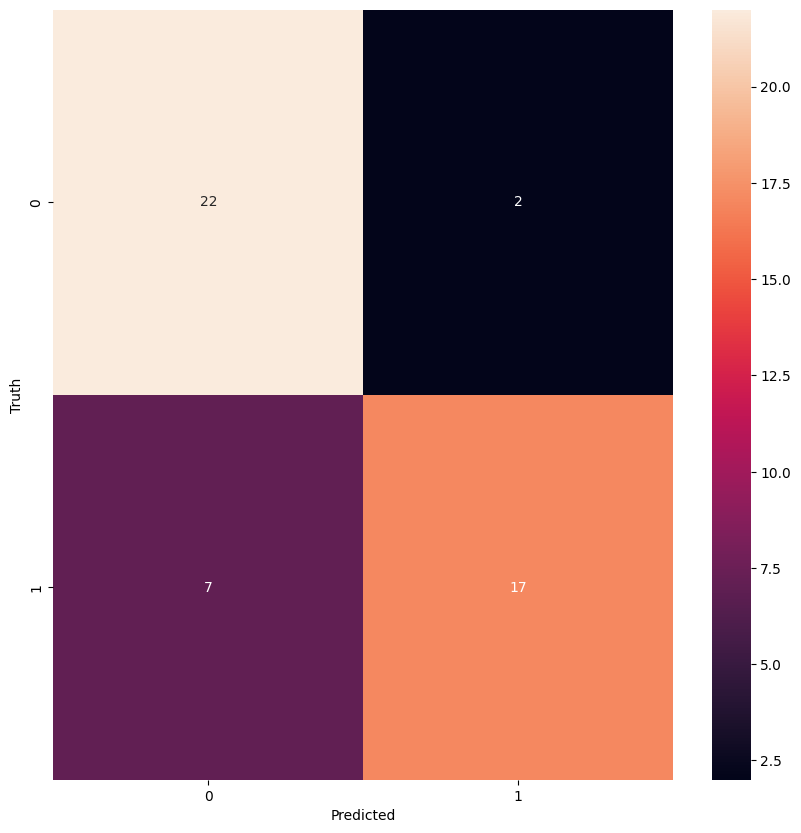
Figure 4: Confusion matrix for random forest model using tsfresh extracted features
Perform a cross validation training:
ts_fresh_accuracies = cross_val_training(df_training.drop("Time_series",axis=1)[selected_features],
                                df_training["Time_series"],
                                RandomForestClassifier(),
                                n_iterations=10
                               )

ts_fresh_mean_accuracies = sum(ts_fresh_accuracies) / len(ts_fresh_accuracies)

print(f"Average of accuracy : {ts_fresh_mean_accuracies}")

#Average of accuracy : 0.8729166666666668
Seglearn
This python package focuses on segmenting time series into homogeneous regions, extracting features from those segments, and using those features for classification or regression tasks.
Seglearn provides a range of tools for time series segmentation and feature extraction, such as piecewise linear approximation (PLA), piecewise aggregate approximation (PAA), and sliding window segmentation. It’s equipped with several feature extraction methods, such as time domain statistics, frequency domain statistics, and wavelet coefficients.
Here is an example of using Seglearn in real case:
Import libraries:
from seglearn.transform import Segment, FeatureRep, FeatureRepMix
from seglearn.feature_functions import minimum, maximum
from seglearn.base import TS_Data
from seglearn.feature_functions import all_features
from seglearn.transform import FeatureRep
import seglearn
Feature extraction: in this part, we will extract features using seglearn. At first Seglearn divide the data frame into slice or segment of size (200 in our case) then it will create a matrix containing one data segment in each row. In the second step, it will extract the features of each segment (each row of the matrix).
def extract_feature_seglearn(df,column_name,segment_width=200,segment_overlap=0):
    X=[]
    X.append(np.array(df[column_name]))

    segment = Segment(width=segment_width, overlap=segment_overlap)
    X, y, _ = segment.fit_transform(X, y=None)

    fs = FeatureRep(features=all_features())

    X = fs.fit_transform(X, y)

    df = pd.DataFrame(data=X, columns=fs.f_labels)

    return(df)

f_amzn_features = extract_feature_seglearn(df_amzn,"value")
df_appl_features = extract_feature_seglearn(df_appl,"value")

df_amzn_features["Time_series"] = 0
df_appl_features["Time_series"] = 1

df = pd.concat([df_appl_features, df_amzn_features], ignore_index=True)
Select the most important features: here we select the most explanatory variables using the importance matrix. we select 20 variables.
X_train, X_test, y_train, y_test = train_test_split(df.drop("Time_series",axis=1), df["Time_series"], test_size=0.3, stratify=df["Time_series"])
clf = RandomForestClassifier()
clf.fit(X_train,y_train)

importances = clf.feature_importances_
indices = np.argsort(importances)

fig, ax = plt.subplots(figsize=(16, 10))
ax.barh(range(len(importances)), importances[indices])
ax.set_yticks(range(len(importances)))
_ = ax.set_yticklabels(np.array(X_train.columns)[indices])

selected_features = list(np.array(X_train.columns)[indices[::-1][:20]])
X_train, X_test = X_train[selected_features], X_test[selected_features]
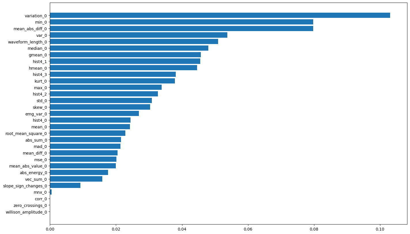
Figure 5: Feature importances extracted by Seglearn
Train a Random forest model:
param_grid = {'max_depth': [2,3,5,10,15,20,50], 'max_leaf_nodes': [2,5,10,15,20], 'min_samples_leaf': [2,5,10],'min_samples_split':[2,5,10,12,15],"n_estimators": [16,32,64, 128, 256,512]}
acc_rf_seglearn = train_evaluate_model(X_train, y_train, X_test, y_test, RandomForestClassifier(), param_grid)
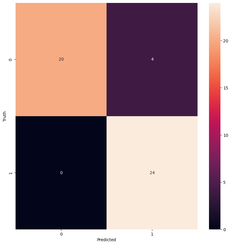
Figure 6: Confusion matrix for random forest model using seglearn extracted features
Perform cross validation training:
seglearn_accuracies = cross_val_training(df.drop("Time_series",axis=1)[selected_features],
                                df["Time_series"],
                                RandomForestClassifier(),
                                n_iterations=10
                               )

seglearn_mean_accuracies = sum(seglearn_accuracies) / len(seglearn_accuracies)

print(f"Average of accuracy : {seglearn_mean_accuracies}")

#Average of accuracy : 0.8687499999999998
Pyts
Pyts is specifically designed for time series classification. It provides various time series classification algorithms such as KNeighborsClassifier, Timeseries Forest, Timeseries Bag-of-Features.
It’s equipped with preprocessing, transformation functions, decomposition and approximation algorithms like Singular Spectrum analysis, Piecewise Aggregate Approximation, Discrete Fourier Transform, …
Since tsfresh and Seglearn extract statistical and autocorrelation features, Pyts suggets more advanced and powerful techniques for feature extraction that we will see in detail below.
- Shapelet Transform: It is a feature extraction technique that relies on shapelets. A shapelet is a consecutive subsequence of a timeseries. This function first extracts the n most discriminative shapelets based on a criterion and returns the distances between the shapelets and the dataset.
- Bag Of Patterns: This function transforms each time series into a bag of patterns using the bag of words algorithm for time series. It consists of extracting subseries using sliding window, transforming each subseries into a word applying Piecewise Aggregate Approximation and Symbolic Aggregate Approximation algorithms. The bag of patterns computes the frequency of each word and transforms each time series into a histogram. The frequency of each word is used as a feature of the time series.
- Bag of Symbolic Fourier Approximation Symbols (BOSS): The BOSS function follows the same principle as Bag of Patterns but it uses Symbolic Fourier Approximation algorithms to extract words. The Symbolic Fourier Approximation combines Discrete Fourier Transform – extracting Fourier coefficients – and Multiple Coefficient Binning – discretization techniques -.
- Word Extraction for TimeSeries Classification (WEASEL): WEASEL follows the same principle as Bag of Patterns and BOSS but instead of using single sliding window, it uses several sliding windows of varied sizes and selects the most discriminative words applying the chi-squared test.
- Random Convolutional Kernel Transform (ROCKET): This is a technique that employs a diverse set of randomly generated convolutional kernels. It extracts two essential features from these convolutions: The maximum value and the proportion of positive values.
Here is an example of using Pyts in real case:
Import libraries:
from pyts.transformation import ShapeletTransform
from pyts.transformation import BOSS
from pyts.transformation import WEASEL
from pyts.transformation import ROCKET
Read the data:
def truncate_data(df):
    subseq_len = 200
    subseq_list = []
    y = []

    for i in range(0, len(df)-subseq_len+1, subseq_len):
        subseq = df['value'].iloc[i:i+subseq_len]
        subseq_list.append(subseq.values)
        y.append(df['Time_series'].iloc[i+subseq_len-1])

    X = np.array(subseq_list)
    y = np.array(y)

    return X, y

df_appl = pd.read_csv(apple_path, sep=",", on_bad_lines='skip')
df_amzn = pd.read_csv(amazon_path, sep=",", on_bad_lines='skip')

df_appl['Time_series'] = 0
df_amzn['Time_series'] = 1


X_apple, y_apple = truncate_data(df_appl)
X_amazon, y_amazon = truncate_data(df_amzn)

X = np.concatenate([X_apple, X_amazon])
y = np.concatenate([y_apple, y_amazon])

X.shape, y.shape
Feature extraction:
def extract_bunch_of_pyts_features(X, y):
  # Shapelet Transform
  print("Computing Shapelet Transform")
  st = ShapeletTransform(n_shapelets=20, n_jobs=-1)
  X_shapelet = st.fit_transform(X, y)

  # BOSS
  print("Computing Boss")
  boss = BOSS(sparse=False)
  X_boss = boss.fit_transform(X)

  #WEASEL
  print("Computing WEASEL")
  weasel = WEASEL(sparse=False)
  X_weasel = weasel.fit_transform(X,y)

  #ROCKET
  print("Computing ROCKET")
  rocket = ROCKET(n_kernels=20)
  X_rocket = rocket.fit_transform(X)

  # Concatenating all exctracted features
  X_final = np.concatenate([X_shapelet, X_boss, X_weasel, X_rocket], axis=1)

  print(f"Shape of final X : {X_final.shape}")

  return X_final, y

X_features, y = extract_bunch_of_pyts_features(X, y)
Select the most important features:
X_train, X_test, y_train, y_test = train_test_split(X_features, y, test_size=0.3, stratify=y)
clf = RandomForestClassifier()
clf.fit(X_train ,y_train)

importances = clf.feature_importances_
indices = np.argsort(importances)

X_train, X_test = X_train[:, indices[::-1][:40]], X_test[:, indices[::-1][:40]]
Train a Random forest model:
param_grid = {'max_depth': [2,3,5,10,15,20,50], 'max_leaf_nodes': [2,5,10,15,20], 'min_samples_leaf': [2,5,10],'min_samples_split':[2,5,10,12,15],"n_estimators": [16,32,64, 128, 256,512]}
acc_rf_pyts = train_evaluate_model(X_train, y_train, X_test, y_test, RandomForestClassifier(), param_grid)
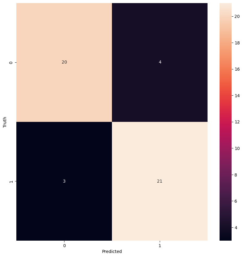
Figure 7: Confusion matrix for random forest model using pyts extracted features
Perform cross validation training:
pyts_accuracies = cross_val_training(X_features[:, indices[::-1][:40]],
                                y,
                                RandomForestClassifier(),
                                n_iterations=10
                               )

pyts_mean_accuracies = sum(pyts_accuracies) / len(pyts_accuracies)

print(f"Average of accuracy : {pyts_mean_accuracies}")
##Average of accuracy : 0.8708333333333333
Comparison of Packages
To help users choose the best package for their needs, we compared tsfresh, seglearn, and pyts based on their features, functionality, and performance. We can see below a comparative table:
| Feature Extraction Library | Description | Supported Data Formats | Feature Extraction Methods | Number of Features | Parallelizable |
|---|---|---|---|---|---|
| tsfresh | Automated feature extraction and selection library for time series data. | Pandas DataFrame with columns ['id', 'time', 'feature_1', 'feature_2', ...] | Statistical, Fourier, Autoregression, Binary, Value count, and additional feature extractors | Hundreds of features | Yes, via Dask or multiprocessing |
| seglearn | Feature extraction library for segmenting and extracting features from time series data. | NumPy arrays with shape (n_samples, n_features) or (n_samples, n_timestamps, n_features) | Mean, variance, slope, change, autocorrelation, FFT, and more feature extractors | Several dozen features | Yes, via joblib or multiprocessing |
| Pyts | Library dedicated to time series classification but containing feature extraction function | Numpy arrays or pandas dataframe | Shapelet Transform, Bag of Patterns, BOSS, WEASEL, ROCKET | Hundreds of features | Yes, via joblib or multiprocessing |
Conclusion
Feature extraction is an important step in time series analysis, as it helps to extract the explanatory variables and make it more interpretable. There are several open-source packages available for time series feature extraction, each with their own strengths and weaknesses. By understanding the different types of features and techniques available, users can choose the best package for their needs and perform more accurate and efficient time series analysis.
all_accuracies = [ts_fresh_accuracies, seglearn_accuracies, pyts_accuracies]


fig, ax = plt.subplots()
ax.boxplot(all_accuracies)


ax.set_xticklabels(['Ts fresh', 'Seglearn', 'Pyts'])
ax.set_ylabel('Accuracy')

# Set a title for the plot
ax.set_title('Comparison of Accuracies')

# Show the plot
plt.show()
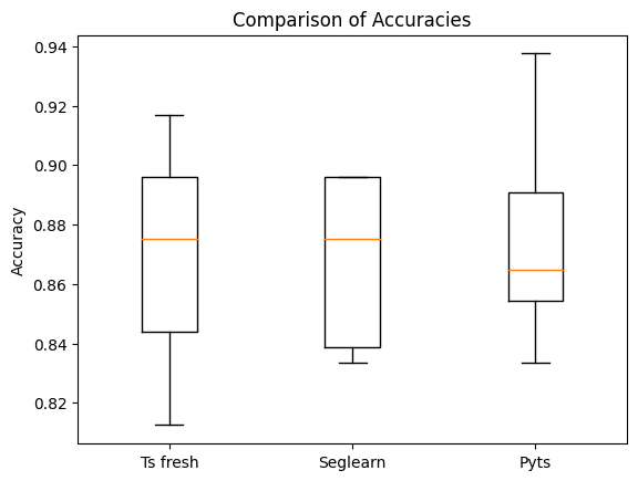
Figure 8: Comparison of accuracies of different feature extraction libraries

Data Scientist at Quantmetry
I am Data Scientist with strong interest in computer vision and time series.

Data Engineer at Quantmetry
Passionate about the field of data, its scientific, technical and business challenges. My current position at QM allows me to continue to explore data engineer tools and data science approaches, push my limits and improve my knowledge.