Quant Blog Le blog des Experts Data & IA

IA de confiance, Machine Learning, Recherche et développement

10/02/2023

Data Augmentation: How do GANs synthesize tabular data in recent studies?

Temps de lecture : 15 minutes

“Data is the new oil” by Clive Humby highlights the importance of data in the 21^st century. In this context, data augmentation is one of the AI trends which solves the lack of data for machine learning tasks. It is even more critical when collecting large amounts of data is difficult, especially for tabular data. Moreover, synthetic data help to protect private information contained in the original data (e.g., medical records) while sharing it with other parties and the research community. Existing applications of synthetic data include deepfake[1], oversampling for imbalanced data, and public healthcare records.

More recently, generative models have emerged as the state-of-the-art technique in generating synthetic data, by discovering the pattern of the original data and generating new samples similar to the original data. In this article, we explore several recent studies on one of the most popular generative architectures, i.e., Generative Adversarial Network (GAN), for generating synthetic tabular data. We also discuss the challenges of the tabular data generation task and how GANs overcome these obstacles.

I. Overview of GANs

GANs are based on a game-theoretic scenario between two neural networks: a generator and a discriminator (Goodfellow, et al., 2016). The generator is a directed latent variable model deterministically generating synthetic samples from noise and tries to fool the discriminator. On the other hand, the discriminator distinguishes between real and synthetic samples of the generator (see Figure 1).

We show a notation of GANs:

Discriminator $D_\phi$ : a neural network with parameters $\phi$
Generator $G_\theta$ : a neural network with parameters $\theta$

The objective of a vanilla GAN is $\min_\theta max_\phi v(G_\theta, D_\phi)$ where:

$v(G_\theta, D_\phi) = E_{x \sim p_{data}} \log D_\phi (x) + E_{z \sim p(z)} \log (1 - D_\phi (G_\theta (z)))$

$x$ is sampled from the real distribution $p_{data}$ .
z is noise, and the generator learns to generate samples from this noise.
$D_\phi (x)$ returns the probability of being a real sample.
$E_{x \sim p_{data}}$ and $E_{z \sim p(z)}$ are respectively the expectation with sampled from data distribution and the expectation with z sampled from its noise distribution

For this GAN, the generator tries to increase the probability of a synthetic sample $D_\phi (G_\theta (z))$ , which means

$\min_\theta v(G_\theta, D_\phi) = E_{z \sim p(z)} \log (1 - D_\phi (G_\theta (z))).$

On the other hand, the discriminator tries to increase the probability of a real sample and decrease the probability of the synthetic sample,

$\max_\phi v(G_\theta, D_\phi) = E_{x \sim p_{data}} \log D_\phi (x) + E_{z \sim p(z)} \log (1 - D_\phi (G_\theta (z))).$

Note that there are several variants of GAN, e.g., Wasserstein GAN (Arjovsky, et al., 2017), PacGAN (Lin, et al., 2017), PATE-GAN (Jordon, et al., 2019), etc., which help to improve the performance of the vanilla GAN.

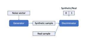
Figure 1: GAN structure.

II. Synthetic table generation task

Tabular data are data structured into a table form. It consists of columns and rows standing for attributes and data samples, respectively. These attributes can depend on one another and have different data types (i.e., categorical and numerical data).

The task of synthesizing tabular data is to generate an artificial table (or multiple relational tables) based on an original tabular dataset. The synthetical table must share similar properties to the original dataset. In practice, it must satisfy the two following properties:

A machine learning task on real and synthetical data must share similar performance.
Mutual dependency between any pair of attributes must be preserved. Note that every sample of synthetic data must differ from the original data.

Generation task notation

We present the notation of the generation task used in (Xu, et al., 2019). In this work, we apply GANs to learn from a single table and generate a single synthetic table.

Input: an original table consists of variables (i.e., columns): continuous random variables (i.e., numerical data) and discrete random variables (i.e., categorical data, ordinal data). Note that these variables follow an unknown joint distribution. independent samples (i.e., rows) come from this joint distribution.
- Columns:
  - $n_c$ continuous random variables: $\{ C_1, \cdots , C_i, \cdots , C_{n_c} \}$
  - $n_d$ discrete random variables: $\{ D_1, \cdots , D_i, \cdots , D_{n_d} \}$
- Row of size n at j^th: $\{ c_{1,j}, \cdots , c_{n_c,j}, d_{1,j}, \cdots , d_{n_d, j} \}$
- Joint distribution: $P(C_{1:n_c}, D_{1:n_d})$
Output: a synthetic table $T_{syn}$
Generative model: $M(C_{1:n_c}, D_{1:n_d})$ produces $T_{syn}$

III. Challenges of tabular data generation

Different types of data

A typical table has different types of data e.g., date-time, real numbers, or categories. Recall that synthetical data must preserve relationships of features. A generative model must learn any dependency between any pair of attributes with different data types, e.g., numerical and categorical data. Moreover, GANs must use different activation functions for the last layer, e.g., “softmax” and “tanh”.

Different distribution forms

Values of the attributes can be sampled from various distribution forms. E.g., multimodal, long tail, non-Gaussian distribution, etc. Our model must memorize all distribution forms in the original table and generate all attributes from these distributions for one sample. Note that some of them are difficult to be learned by GANs: normalization of non-Gaussian data (e.g., min-max transformation) can easily cause a vanishing gradient problem(Xu, et al., 2018), and a vanilla GAN hardly models the multimodal distribution of continuous variables (Srivastava, et al., 2017; Xu, et al., 2019).

Imbalanced categorical data

For categorical data, we can see a common issue called “Imbalanced categorical data” in that the categories are not represented equally. In this case, the discriminator struggles to distinguish samples of minor categories, e.g., it can assign these samples to fake samples. This is more important when generating synthetical data for a classification task.

Generation of multi-tables in a database

The task also handles multiple relational tables. In detail, a table contains at least one unique attribute called “key” which allows each row in this table to be uniquely identified and references to a row of another table. In this case, the generative model produces a list of synthetic relational tables that preserve their mutual relationships.

IV. Components for generating tabular data in GANs

In this section, we show several components used recently in GANs to overcome the challenges of tabular data generation: preprocessing methods, conditional generators, and objective function components. The preprocessing methods help to transform tabular data into neural network inputs with a suitable format. We also see how GANs produce samples for minor categories with a conditional generator. Finally, objective function components improving synthetic data quality are discussed.

IV.A. Preprocessing

For the preprocessing step, we need several reversible transformations which allow data to be efficiently fitted by a neural network model. In the case of numerical attributes, a normalization method should be applied. For example, (Xu, et al., 2019) converted these attributes into scalars ranging in $(-1, 1)$ since they use the “tanh” activation function[2] for their neural networks. For categorical attributes, we can use one-hot-encoding and a “softmax” activation function[3] to generate probabilities of their categories.

IV.A.1. Mode-specific normalization for numerical data and mixed data

(Xu, et al., 2018) found that a simple normalization scale can lead to saturating gradient problem (Goodfellow, et al., 2016). Moreover, the datasets used in their paper consist of attributes containing multiple modes. They proposed to cluster values of a numerical attribute by using a gaussian mixture model[4] (i.e., its distribution is a weighted sum of $m$ multiple modes). For this approach, a numerical attribute is represented by a one-hot vector of size $m$ showing the probabilities of $m$ modes and a scalar showing its value for the highest probability mode.

(Zhao, et al., 2021) extended this normalization method for mixed data type[5] (Sahoo, et al., 2020), i.e., the random variable consists of both continuous and categorical values, or continuous values and missing values. The value of this variable should be equitably sampled from both distribution elements. For this normalization method, they add a binary standing for categorical modes (or missing value mode) in the one-hot vector. An example is found in Figure 2. These methods can help to simplify a complex distribution. However, (Mottini, et al., 2018) found that using Gaussian mixture models for numerical attributes reduces the quality of synthetic data.

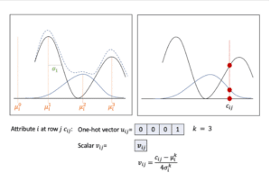
Figure 2: Mode-specific normalization for $c_{ij}$ : mixed data attribute (i.e., missing $\mu_i^0$ and continuous values $\mu_i^1$ , $\mu_i^2$ and $\mu_i^3$ ) at row $j$ .

IV.A.2. Smoothing for categorical variables

In (Xu, et al., 2018; Xu, et al., 2019), noise is added into one-hot categorical representations to remove their sparsity. They add uniform noise $\mathcal{N}(0, \gamma)$ (e.g., $\gamma=0.2$ ) to each cell of these one-hot vectors, and then renormalize the noised representations (see Figure 3). Note that we can avoid adding noise by using cross-networks introduced by (Wang, et al., 2017). (Mottini, et al., 2018; Engelmann, et al., 2020) use these networks to transform directly one-hot vectors into continuous vectors.

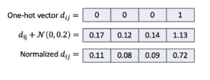
Figure 3: Smoothing for a categorical attribute $d_{ij}$

IV.A.3. Logarithm transformation

(Zhao, et al., 2021) proposed a logarithm transformation (FENG, et al., 2014) to deal with skewed data or long-tail distribution[6] since Gaussian mixture models hardly fit the data towards the tail. Given a lower bound $l$ and a noise $\epsilon$ , they replace any initial value $\tau$ lower than this bound by a compressed value $\tau^c$ :

$\tau^c \begin{cases} \log(\tau) \text{ if } l > 0 \\ \log(\tau - l + \epsilon) \text{ where } \epsilon > 0 \text{ if } l \leq 0\end{cases}$

This method reduces the skewness (i.e., the distance between the tail and bulk data), which helps Gaussian mixture models to encode tail values. An example of its effect is in Figure 4.

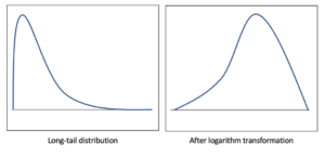
Figure 4: Long-trail distribution before (left figure) and after logarithm transformation (right figure).

IV.B. Conditional Generators

Conditional GANs, introduced by (Mirza, et al., 2014), are constructed by feeding categorical attributes to both the generator and discriminator. They generate the rest of the features based on these categorical input attributes. This helps to rebalance the imbalanced categorical data, by generating samples for minority categories (Xu, et al., 2018; Xu, et al., 2019; Zhao, et al., 2021; Engelmann, et al., 2020). An example of a conditional generator is displayed in Figure 5.

During training, a conditional attribute is uniformly selected. A category of this conditional feature is then selected based on the logarithm of their probabilities (i.e., frequency), which gives minor categories higher chances to sample. This approach is called “training-by-sampling” (Xu, et al., 2019) (see Figure 9). For $n$ categorical attributes, a conditional input vector is simply a concatenation of $n$ one-hot vectors of these attributes, where the cell of the selected category (of the selected feature) is set to 1. We can apply this approach to continuous skewed data by selecting minor modes after mode-specific normalization. We can notice that tackling data imbalance improves the performance of the discriminator, and in general, it returns correct feedback for the generator.

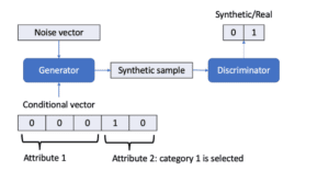
Conditional generator with a conditional vector

Figure 5: Conditional generator with a conditional vector. There are two categorical attributes in this example data and the generator produces a synthetic sample for category 1 of attribute 2.

IV.C. Classifier for semantic integrity

(Park, et al., 2018; Zhao, et al., 2021) concentrated on preserving correlations between categorical attributes and others. For each feature, a neural network classifier $C$ pre-trained on the original data gives feedback to the generator: a categorical feature is predicted based on the rest of the features. In this case, the loss of a classifier means the discrepancy between the generated category and the category predicted by the classifier. This loss is added to the main objective function of GANs:

$L_{class}^G = E_{z \sim p(z)} (| l(G(z)) - C(remove(G(z))) |)$

where $remove()$ removes the label of an attribute for a sample and $l()$ returns this label. Note that these classifiers can share the same intermediate layers. (Zhao, et al., 2021) confirmed that this approach improves machine learning efficacy.

IV.D. Information loss

Besides classification loss, (Park, et al., 2018) also introduced information loss which is the distance between the synthetic and original data. It measures how close synthetic data is to the original one, which shows the privacy of the synthetic data. In detail, this loss matches the mean $E$ and the standard deviation $SD$ of each sample. This loss is also added to the main objective function of GANs. (Park, et al., 2018; Zhao, et al., 2021) proved that it improves training stability since it guides the generator to reconstruct ground-truth values.

$L_{mean} = || E_{x \sim p_{data} f(x)} - E_{z\sim p(z)} f(G(z))||_2$

$L_{sd} = || SD_{x \sim p_{data} f(x)} - SD_{z\sim p(z)} f(G(z))||_2$

where $f()$ returns the features fed into the softmax layer of $D$ .

V. Recent studies

In this section, we discuss several remarkable variants of GAN such as MedGAN, Table-GAN, TGAN/CTGAN, and CTAB-GAN. Most of the models apply the components mentioned in the previous section to overcome the challenges of generating synthetic tables e.g., data with different types, long tail/multimodal distribution, and imbalanced data.

MedGAN

MedGAN, proposed by (Choi, et al., 2017), generates discrete attributes of patient records (e.g., binary and count features). Recall that the vanilla GAN only processes continuous variables. To overcome this limitation, they pre-train an autoencoder (Goodfellow, et al., 2016) on the original data. Basically, an autoencoder is built to reconstruct the input samples:

- first it compresses data via an encoder projecting them into lower dimensional space,
- then it expands the information via a decoder projecting them back to the input space.

This decoder helps to transform the continuous output of the generator (a feedforward neural network) into discrete variables (Figure 6). These variables are then fed into the discriminator. They also found that the discriminator trained without explicit rounding of these variables gives better performance than with rounding.

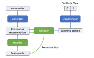
Figure 6: In MedGAN, the decoder $Dec()$ of the autoencoder (reconstructing the input) is reused to transform the continuous output of the generator into the original format (i.e., a synthetic sample with discrete variables).

Table-GAN

Table-GAN of (Park, et al., 2018) focuses on privacy and semantic integrity. Therefore, they introduced information loss (see D) to control the privacy level of the generated data and the loss of classifiers (see V.C) to preserve correlations between categorical features and the rest of the features. To control privacy, they added a threshold of the mean $\delta_{mean}$ and the standard deviation $\delta_{sd}$ of features into the information loss.

$L_{info}^G = \max(0, L_{mean} - \delta_{mean}) + \max(0, L_{sd} - \delta_{sd})$

Different from MedGAN, this model is based on convolutional neural networks (CNNs)(Goodfellow, et al., 2016) where a sample is represented by a matrix of features. In detail, the generator includes deconvolutional layers (i.e., from a noise vector to a matrix of features) and the discriminator includes convolutional layers (i.e., from the matrix of features to a probability), as shown in Figure 7. They concluded that CNNs can help to capture the correlations between features. However, it is unclear whether different matrix representations (i.e., different orders of the attributes) return the same generation performance. Based on their experiments, they found that using the original vector format leads to a sub-optimal performance due to its limited convolution computations.

Table-GAN based on CNNs

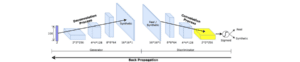
Figure 7: Table-GAN based on CNNs: the generator and the discriminator follow deconvolution and convolution processes, respectively. Source: (Park, et al., 2018).

TGAN and CTGAN

TGAN (Xu, et al., 2018) generates features one by one (following their original order in the table) by using an LSTM[7] (Hochreiter, et al., 1997; Graves, 2013; Goodfellow, et al., 2016). These models use mode-specific normalization for numerical data (see A.1) and smoothing for categorical data (see V.A.2). In this case, the LSTM-based generator returns these values $v_{1:n_c,j}, u_{1:n_c,j}, d_{1:n_d,j}$ one by one for each row $j$ . Note that this model also uses an attention mechanism $a_{1:n_c}, a_{1:n_c}, a_{1:n_d}$ to weight the relationships between the current attribute to the previously generated features. An example of TGAN is displayed in Figure 8.

example of TGAN

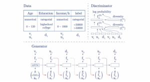
Figure 8: An example of TGAN for two numerical features and two categorical features. The model generates each component of numerical features and a value of categorical features one by one. Each output (e.g., $d_1$ ) is based on a noise vector $z$ , the previously generated output (e.g., the representation before activation function ), and an attention matrix (e.g., $a_2$ ). $v$ and $u$ are the two elements for a numerical attribute (mode-specific normalization) and $d$ stands for a categorical attribute. Source: (Xu, et al., 2018).

Considering tabular data as a sequence of features by using LSTM is computationally less efficient and does not perform better than a simple feedforward neural network (Engelmann, et al., 2020). Moreover, the lack of an appropriate order of generating features can lead to an incorrect correlation between them. Therefore, their follow-up CTGAN (Xu, et al., 2019) uses feedforward neural networks for their generator and their discriminator. Moreover, it is based on the Wasserstein GAN, which improves the performance of the GAN (Arjovsky, et al., 2017). CTGAN also includes a conditional generator, tackling the data imbalance. We show the architecture of CTGAN in Figure 9.

CTGAN architecture

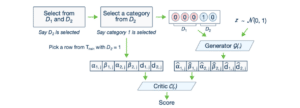
Figure 9: CTGAN architecture. Critic C(.) replaces the role of the discriminator for Wasserstein GAN. We can see how a conditional vector is constructed. $D_1$ and $D_2$ are categorical attributes. $\alpha$ and $\beta$ are the two elements for a numerical attribute (mode-specific normalization) and $d$ stands for a categorical attribute. Source: (Xu, et al., 2019).

CTAB_GAN

CTAB-GAN of (Zhao, et al., 2021) uses an extended version of mode-specific normalization, which processes the mixed data. It includes a classifier (a feedforward neural network) for semantic integrity and computes the information loss to improve training stability. The generator and the discriminator are based on the architecture of Table-GAN (i.e., CNNs).

In addition, we should mention the work of (Engelmann, et al., 2020): their CWGAN is based on a conditional Wasserstein GAN (Arjovsky, et al., 2017) and a cross-network (Wang, et al., 2017) for data oversampling. (Rajabi, et al., 2021) would like to improve the fairness in data (e.g., all genders should have a similar salary). The objective function of their model TabFairGAN includes fairness constraints: penalizing the difference of an attribute (e.g., salary) between different categories (e.g., female and male).

VI. Conclusions

In this article, we explored the components used in recent studies that help GANs overcome the challenges in tabular data generation.

Mode-specific normalization and smoothing methods are for pre-processing different data types, which helps GANs to easily learn tabular data.
Conditional generators and the training-by-sampling improve the data generation performance by rebalancing the data input.
Classification and information loss help to preserve feature correlation, control data privacy and improve training stability.

These recent studies broaden the ability of GANs in data augmentation. In fact, collecting large-size tabular data is hard and time-money consuming, especially medical records and customer data. GANs can produce good-quality synthetic data for under-resourced applications. This can improve the performance of machine learning models and reduce the problem of imbalanced and skewed data. Many clients of Quantmetry must deal with their low-resource data, hence GANs open a highway to overcome the lack of data and enhance the performance of their tasks.

One remaining challenge is the generation of multi-tables in a database, where GANs can handle unique keys (i.e., it must learn how all the attributes from all the generated tables are related through these keys). Another difficult problem is how to add constraints into synthetic data e.g., an attribute must be positive, negative, or in an interval; all values of an attribute are always larger/smaller than the values of another attribute; etc. More work is needed there to design GAN components and generation strategies that overcome these obstacles.

I would like to extend my sincere thanks to Ali JABBARI, Grégoire MARTINON, Cyril LEMAIRE, Louis LACOMBE, and Geoffray BRELURUT for constructive criticism of this blog article.

VII. Bibliography

Goodfellow Ian, Bengio Yoshua and Courville Aaron Deep Learning [Book]. – [s.l.] : MIT Press, 2016.

Xu Lei [et al.] Modeling Tabular Data using Conditional GAN [Conference]. – 2019.

Zhao Zilong [et al.] CTAB-GAN: Effective Table Data Synthesizing [Conference]. – 2021.

Sahoo Saswata and Chakraborty Souradip Learning Representation for Mixed Data Types with a Nonlinear Deep Encoder-Decoder Framework [Journal]. – 2020.

Srivastava Akash [et al.] VEEGAN: Reducing Mode Collapse in GANs using Implicit Variational Learning [Conference] // NIPS. – 2017.

Xu Lei and Veeramachaneni Kalyan Synthesizing Tabular Data using Generative Adversarial Networks. – 2018.

Wang Ruoxi [et al.] Deep & Cross Network for Ad Click Predictions [Conference] // AdKDD and TargetAd. – 2017.

Mottini Alejandro, Lheritier Alix and Acuna-Agost Rodrigo Airline Passenger Name Record Generation using Generative Adversarial Networks [Conference] // ICML 2018 – Workshop on Theoretical Foundations and Applications of Deep Generative Models. – 2018.

Engelmann Justin and Lessmann Stefan Conditional Wasserstein GAN-based Oversampling of Tabular Data for Imbalanced Learning. – 2020.

Mirza Mehdi and Osindero Simon Conditional Generative Adversarial Nets. – 2014.

Park Noseong [et al.] Data Synthesis based on Generative Adversarial Networks [Conference] // VLDB. – 2018.

Arjovsky Martin, Chintala Soumith and Bottou Léon Wasserstein GAN. – 2017.

Lin Zinan [et al.] PacGAN: The power of two samples in generative adversarial networks. – 2017.

Jordon James, Yoon Jinsung and Schaar Mihaela van der PATE-GAN: Generating Synthetic Data with Differential Privacy Guarantees [Conference] // ICLR 2019 Conference. – 2019.

Choi Edward [et al.] Generating Multi-label Discrete Patient Records using Generative Adversarial Networks [Conference] // Machine Learning in Health Care (MLHC). – 2017.

Hochreiter Sepp and Schmidhuber Jürgen Long Short-Term Memory [Conference] // Neural Computation. – 1997.

Graves Alex Generating Sequences With Recurrent Neural Networks. – 2013.

Rajabi Amirarsalan and Garibay Ozlem Ozmen TabFairGAN: Fair Tabular Data Generation with Generative Adversarial Networks. – 2021.

C Feng [et al.] Log-transformation and its implications for data analysis [Journal]. – [s.l.] : Shanghai Arch Psychiatry, 2014.

[1] https://en.wikipedia.org/wiki/Deepfake

[2] https://www.ml-science.com/tanh-activation-function

[3] https://en.wikipedia.org/wiki/Softmax_function

[4] https://scikit-learn.org/stable/modules/mixture.html

[5] A nice presentation about mixed data type: https://www.ima.umn.edu/materials/2018-2019/SW11.7-9.18/27702/Markatou_IMA_November2018.pdf

[6] https://en.wikipedia.org/wiki/Long_tail

[7] https://en.wikipedia.org/wiki/Long_short-term_memory

Les membres de l’expertise Reliable AI développent des modèles performants, fiables et maîtrisés, sur l’ensemble du cycle de vie, pour une IA de confiance.

Anh Khoa NGO HO

Data Scientist chez Quantmetry

PhD in Computer Science and Natural Language Processing. Passionate about Deep Learning and generative models, I work in a research team at Quantmetry which develops state-of-the-art methods to solve industrial problems. I am also part of the trusted AI expertise whose objective is to develop efficient, reliable and controlled models, over the entire life cycle, for trusted AI.