

Generative AI: a guide to evaluate synthetic tabular data

Synthetic tabular data has become increasingly popular in recent years, as it offers a cost-effective answer to data augmentation for machine learning model improvement and sensitive data privacy. However, it is important to ensure that the synthetic data generated is of high quality and accurately represents the real data. To achieve this, it is essential to use reliable evaluation metrics that can assess the similarity and the distance between the synthetic and real data. In this article, we will discuss several widely used evaluation metrics for synthetic tabular data. We will explore how these metrics work, and how they can be applied to evaluate the quality of synthetic data for different types of data features. Understanding these evaluation metrics is crucial for anyone working with synthetic tabular data, as it ensures that the generated data is reliable and effective for training machine learning models.
Experiment Settings
To demonstrate these metrics, we trained three generative models (i.e., CTGAN, TVAE, and CSDI_T) on the Credit dataset (Grinsztajn et al., 2022). This dataset has 13 272 samples, with 22 features (3 categorical features, 19 numerical features). We randomly select 5000 samples for training and use the full dataset for evaluation metric computations. A scatter plot of the real data and its synthetic data for two features is displayed in Figure 1.
- CTGAN and TVAE of (Xu et al., 2019) are based on Generative Adversarial Networks and Variational Autoencoders, Their code can be found in the SDV library.
- CSDI_T (Tashiro et al., 2021, Zheng et al., 2022) is a diffusion model for imputing time-series data (i.e., filling in missing values at a moment based on observed values). We modified this model to generate synthetic tabular data. To obtain a fixed number of synthetic samples, we need to randomly create some observed values for each sample. In detail, we randomly select several features and create values for them. Note that the continuous values must lie between the minimum and maximum values of the real data. For categorical features, the categories of the real data are randomly selected. Other features are considered missing values. The trained diffusion model imputes these missing values.
- Moreover, we also create a vanilla synthetic dataset (called Random for the next sections) as a baseline for these models. For numerical features, we uniformly sample the interval lying between the minimum and maximum observed values. In the case of categorical features, we randomly select categories found in the real data. This means that this kind of dataset has a low correlation between their features.
We use the default hyperparameters to train all the models above. Moreover, we reuse several implementations of metrics found in SDMetrics.
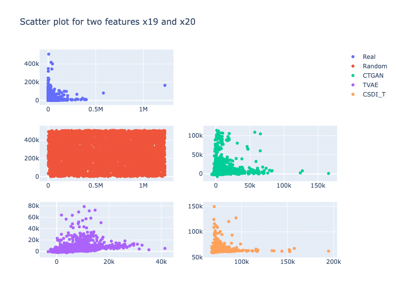
Figure 1: Scatter plot of the real data and its synthetic datasets, for two features 19 and 20. We can see that the relationship between the two features, generated by CSDI_T is close to the counterpart of the real data. In the case of CTGAN, the relationship pattern seems to be enlarged while TVAE fails to preserve this relationship.
Statistical metrics for a quick evaluation
In this section, we discuss several widely used statistical metrics: statistical tests, distance metrics, correlation metrics, and coverage metrics. In this family of metrics, we compare the real data and its synthetic counterpart for each feature. The overall score is then calculated as the mean of the feature-wise scores, resuming the multivariate problem to a sum of univariate ones. These metrics are easily computed and quickly give us an overview of the quality of synthetic data.
Statistical tests
For this kind of metric, we can use the chi-square test and the Kolmogorov-Smirnov test (their implementations are found in SDMetric). The Chi-square test compares the distribution of a categorical feature in the real dataset and the synthetic dataset. It uses the p-value, which indicates the probability that the two distributions were drawn from the same underlying population. On the other hand, the Kolmogorov-Smirnov test evaluates the distribution of numerical features in real and synthetic datasets, comparing their cumulative distribution functions. The score is computed as 1 minus the KS-Test D statistic (the code to compute the KS-Test D statistic can be found in the library Scipy), which represents the maximum distance between the expected and observed cumulative distribution function values. Higher scores on the Kolmogorov-Smirnov test, and better quality of the generated data.
In Figure 2, all methods obtain very high scores for discrete features (i.e., the p-value of the Chi-Squared test larger than 0.8), which implies that discrete features of the synthetic datasets are not very different from the counterparts of the real data. However, it seems that these discrete features are easy to be captured since a simple method such as Random can also reach this level of performance. We will dig deeper into this unexpected behavior in further articles. For continuous features, TVAE obtains the best score, followed by CTGAN and then CSDI_T. We also observe that our diffusion model CSDI_T fails to learn the continuous features because its score in the Kolmogorov-Smirnov test is too close to the score of the random method.
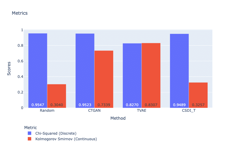
Figure 2: Chi-Squared and Kolmogorov-Smirnov test.
Distance metrics
Another approach is distance metrics. For discrete features, the Jensen-Shannon Distance is commonly used, while the Wasserstein Distance is for continuous features. These distance metrics measure the distance between the probability mass distributions of a categorical or numerical feature in real and synthetic datasets. A small score indicates that the probability mass distributions are similar, and therefore, the quality of the synthetic data for that particular feature is higher. Regarding Figure 3, we see similar patterns of statistical tests in which TVAE obtains the best result for continuous features but the worst performance for discrete features. An explanation is that TVAE only generates a small subset of categories, which leads to a large distance between its synthetic dataset and the real data (see Coverage metrics). This highlights that VAEs work better with continuous features than discrete features.
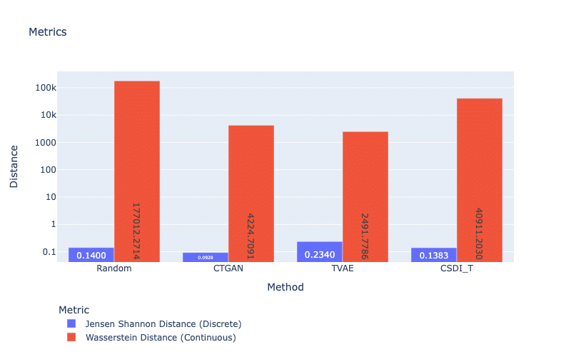
Figure 3: Jensen Shannon and Wasserstein Distance. For both scores, smaller is better.
Correlation metrics
Correlation metrics measure the correlation difference between features in real and synthetic datasets (Zhao et al., 2021). To compute these metrics, we use Chi-squared for discrete features, Pearson for continuous features, and One-way ANOVA (for discrete versus continuous features) to compute the p-values for each pair of features. Our metrics return absolute differences between these p-values of the real and synthetic datasets.
For correlation evaluation, our three models obtain similar scores, except for the correlation score of TVAE using the Chi-squared test (see Figure 4). We also see that TVAE gains the best performance with the smallest scores for all metrics. Recall that TVAE struggles to handle discrete features based on the Jensen-Shannon distance metric. However, TVAE can well preserve the correlation between these features. This could be because of the reconstruction loss of the auto-encoder used in TVAE.
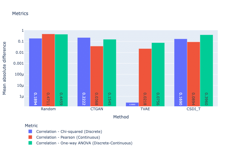
Figure 4: Correlation metrics with Chi-squared, Pearson, and One-way ANOVA tests. For these scores, smaller is better.
Coverage metrics
The coverage metric determines whether a synthetic dataset covers the full range of values (or all categories) present in the real dataset. For these metrics, a score (or a ratio) is equal to 1.0 if the synthetic dataset includes the same range of values or set of categories as the real data (Goncalves et al., 2020, Zhao et al., 2021). Note that this score can be larger than 1.0 because the value ranges or category numbers included in the training set (then learned by our generative models) are larger than the counterparts of the dataset (used for computations of these metrics). In our case, we use the full dataset for metric computations, therefore, the maximum value that can be reached is 1.0.
In Figure 5, we see that CTGAN can cover larger ranges and generate more distinct values than other models (except CSDI_T for discrete features). In contrast, TVAE obtains the lowest performance for both discrete and continuous features. This is because TVAE overfits the training set and loses its generalization (i.e., the model prefers optimizing construction loss to KL divergence).
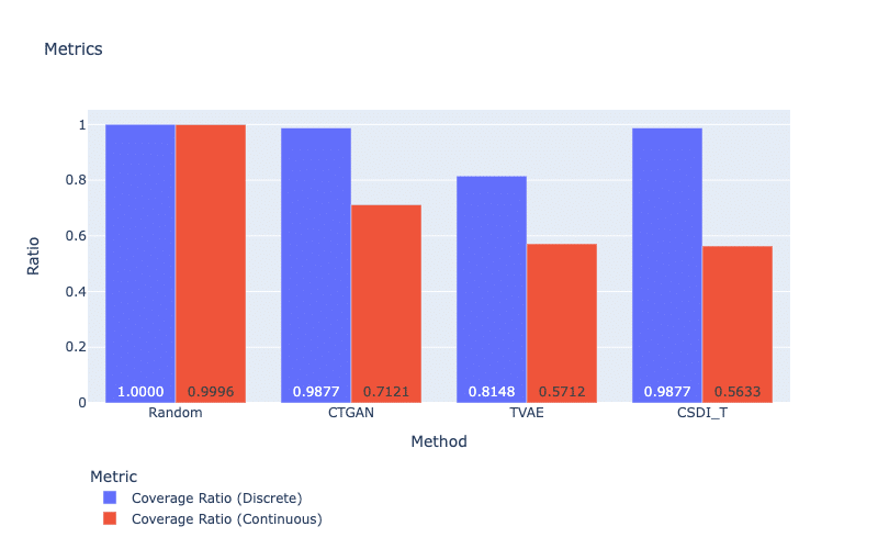
Figure 5: Coverage metrics. For both metrics, a larger score is better.
Indirect evaluation: model-based metrics
For this kind of metric, we need to train a model to obtain evaluation scores. Note that these scores depend on the performance of this metric model and how we train it (i.e., its hyperparameters). Therefore, we use these metrics with caution. In this section, we run through two families of indirect evaluation metrics: likelihood metrics and detection metrics.
Likelihood metrics
Likelihood metrics measure the likelihood that synthetic data is a member of the real data, with a higher score indicating a better quality of the dataset. For example, in SDMetrics, the Bayesian Network of the library Pomegranate is trained on all discrete features of the real dataset, and it computes a log-likelihood score for the discrete features of its synthetic dataset. In the case of continuous features, Multiple Gaussian Mixtures can be used. In Figure 6, we observe likelihood scores using Multiple Gaussian Mixture. This likelihood model gives the largest log-likelihood to TVAE whereas CSDI_T obtains the smallest score. This score of CSDI_T is a sign of a low-quality dataset.
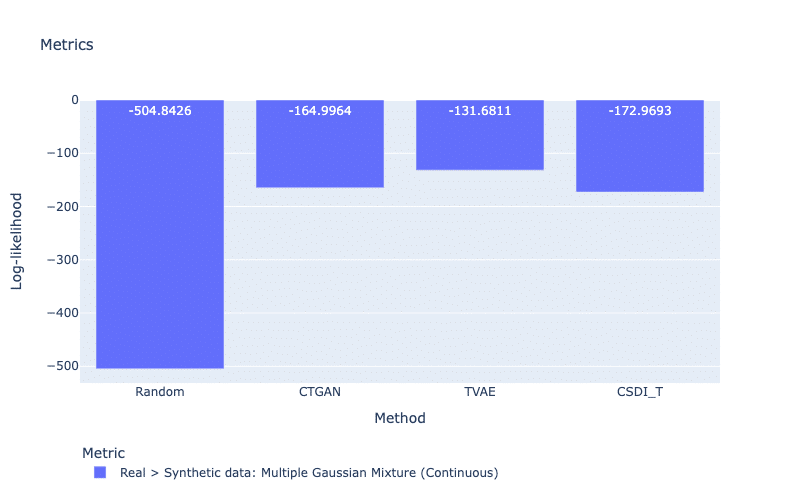
Figure 6: Likelihood metric using Multiple Gaussian Mixtures. For this metric, a larger score is better.
Detection metrics
Detection metrics calculate the difficulty of distinguishing real data from its synthetic counterpart. There are two options: a supervised approach using discrimination classifiers (i.e., discriminator metrics), and an unsupervised approach using clustering algorithms (i.e., clustering metrics). For these metrics, the real data and its synthetic data need to be mixed, then distinguished by the models above. For the former metric, a discriminator assigns each sample to the “Real” or “Synthetic” class and returns a prediction accuracy (e.g., AUC). The metric output is computed as 1 minus AUC under cross-validation, indicating the misclassification of this discriminator. It is equal to 0.0 if this discriminator cannot distinguish between synthetic and real samples, indicating high-quality data.
Figure 7 displays the prediction accuracies of two discrimination classifiers: Logistic Regressor (LR) and SVM Classifier (SVC). We observe that LR and SVC have much more difficulty in correctly assigning the samples generated by TVAE and CTGAN than CSDI_T. In fact, only a small percentage of samples (less than 1%) are correctly classified in the case of CSDI_T. This problem can come from our strategy of generating samples, where we created several known random values and then CSDI_T imputes the missing values.
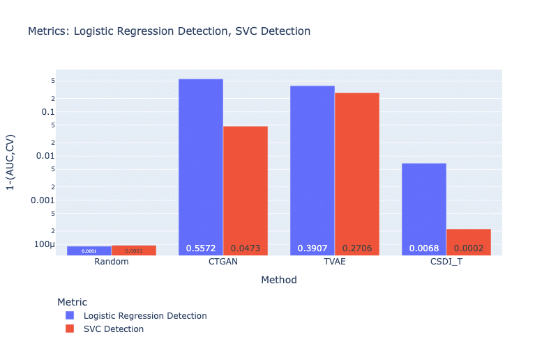
Figure 7: Discriminator metrics. For both metrics, a larger score is better.
On the other hand, the clustering metric assesses how difficult it is to cluster the real and synthetic data into two clusters (by using a clustering algorithm, e.g., K-means clustering). The metric returns the Log-cluster score (proposed by Goncalves et al., (2020), with a smaller score indicating better data quality. Again, we can see that the best result belongs to TVAE.
Quality evaluation for machine learning tasks: Machine learning efficiency metrics
Machine learning (ML) efficiency metrics calculate the success of using synthetic data to perform a ML prediction task (Xu et al., 2019). In other words, if we replace the real data with a synthetic dataset, can we obtain a similar performance? To obtain a metric score, a classifier (or a regressor) is trained on the synthetic dataset to predict a feature based on the rest of the features. The score is computed as the prediction accuracy (e.g., F1 or R2) when we evaluate this model on the real dataset. For this strategy, the metric indicates if a trained model on synthetic data can understand the real data. In our work, MLP, Decision Tree Classifier, and Linear Regression are considered for classification and regression tasks. Figure 9 and Figure 10 display mean prediction accuracy scores for all discrete and continuous features, respectively. In general, TVAE obtains the best scores for both types of features. For discrete features, it is surprising that our generative models do not create large improvements compared with the simple method Random.
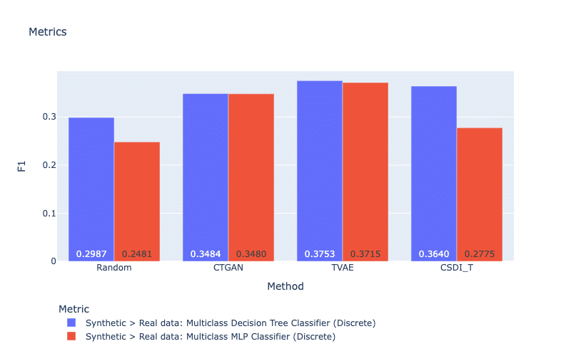
Figure 8: ML efficiency metrics for discrete features. For both metrics, a larger score is better.
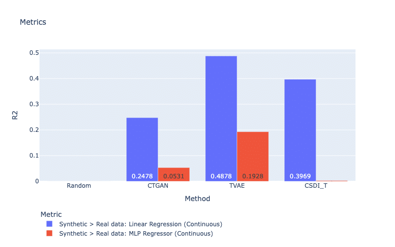
Figure 9: ML efficiency metrics for continuous features. For both metrics, a larger score is better.
Evaluation metrics to ensure the privacy of sensitive information
For sensitive data such as medical records, biometric data, or political opinions, it is important that all sensitive information must be censored if the data are published for the research community. One solution is to publish synthetic data instead of real data. Therefore, we need metrics that allow us to protect sensitive information. In this article, we present two privacy metrics: the Min Distance Pair metric and the Attacker Model metric. For the Min Distance Pair metric, we calculate the distance (e.g., Euclidean distance) between synthetic samples and its closest real samples to ensure that identical samples do not exist (i.e., distance is not equal to 0.0) (Zhao et al., 2021). This is to prevent the generative models from reproducing the same data, which can be a serious privacy concern. For example, if a real record of a patient is found in a synthetic dataset published online (with personal information such as name, home address, and age), this information can be used to trace back this patient. Figure 9 shows that all models do not copy real samples in their synthetic data. Another observation is that samples of TVAE are closest to the real samples, which also demonstrates their higher similarity to the real data than samples of other models.
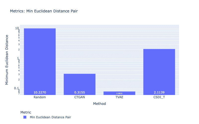
Figure 10: Privacy metric using Euclidean distance. A smaller score is better.
Another approach is the attacker model metric, which measures the success of using synthetic data to recover missing values in the real data. This metric is particularly helpful in scenarios where a sensitive piece of information can be revealed by using a prediction model e.g., the income of a person can be predicted by online transactions. If the prediction model is well-trained on synthetic data, it can correctly predict this piece of information.
To evaluate the effectiveness of the attacker model, we use the same metrics as in the ML efficiency metrics. However, the goal here is to minimize prediction accuracy to ensure that using synthetic data does not help to leak sensitive information. In reality, we can use a threshold to filter out models that do not satisfy the privacy requirements, such as accepting only models with an accuracy lower than a certain value.
How to select the best synthetic dataset based on our list of metrics?
It is a tough question! Let us recall that some metrics do not share the same goal. For example, the ML efficiency metrics and the attacker model metric. The former expects that the same performance of machine learning tasks can be found by using synthetic data. If we use a prediction model trained on synthetic data, it can help recover missing information in real data. This obviously violates the privacy guaranteed by the attacker model metric. Another case is the coverage metrics. In fact, synthetic data that gain better scores in the statistical tests or distance metrics, seem to obtain lower scores in the coverage metrics.
An advice is that we should prioritize metrics that fit well to our problem. The first choice is the statistical metrics so we quickly obtain an overall view of the quality of synthetic data. We also use the likelihood and detection metrics to reinforce our conclusions about data quality. If our synthetic datasets are used for a machine learning task, ML efficiency metrics are definitely essential metrics. If we synthesize medical records, we must concentrate on privacy metrics instead of the best scores in ML efficiency.
Is there a method to combine all metrics? A general method is rank voting: we rank our synthetic dataset and then combine these ranks (e.g., sum or average). Another solution is to count the number of metrics that a model obtains the best score, and the best model wins in most metrics (known as first-past-the-post voting). Chundawat e al. (2022) use the average score of statistics, correlation, detection, and ML efficiency metrics, to obtain a quality score for each synthetic dataset.
Conclusions
In today’s world, where data is the most valuable resource, protecting our personal data has become a primary concern. The introduction of the General Data Protection Regulation (GDPR) in 2018 has emphasized the importance of data privacy and ethical data usage. Synthetic data generation is an effective solution to use data without violating privacy, making it a widespread topic of research. The evaluation metrics discussed in this article play a vital role in ensuring the quality of synthetic data. These metrics not only measure the similarity between real and synthetic data but also prevent sensitive data from leaking. By using these metrics, data scientists can ensure that the synthetic data generated are of high quality and can be used for various machine learning applications. As the use of synthetic data continues to grow, the need for high-quality data will only increase, and evaluation metrics will remain essential to keep data quality intact.
I would like to extend my sincere thanks to Julien ROUSSEL, Hông-Lan BOTTERMAN and Geoffray BRELURUT for constructive criticism of this blog article.
Bibliography
- Grinsztajn, L., Oyallon, E., & Varoquaux, G. (2022). Why do tree-based models still outperform deep learning on tabular data? arXiv. https://doi.org/10.48550/arXiv.2207.08815
- Xu, L., Skoularidou, M., & Veeramachaneni, K. (2019). Modeling Tabular data using Conditional GAN. arXiv. https://doi.org/10.48550/arXiv.1907.00503
- Zheng, S., & Charoenphakdee, N. (2022). Diffusion models for missing value imputation in tabular data. arXiv. https://doi.org/10.48550/arXiv.2210.17128
- Tashiro, Y., Song, J., Song, Y., & Ermon, S. (2021). CSDI: Conditional Score-based Diffusion Models for Probabilistic Time Series Imputation. arXiv. https://doi.org/10.48550/arXiv.2107.03502 . GitHub: https://github.com/ermongroup/CSDI
- Zhao, Z., Kunar, A., Birke, R., & Chen, L. Y. (2021). CTAB-GAN: Effective Table Data Synthesizing. arXiv.https://doi.org/10.48550/arXiv.2102.08369
- Goncalves, A., Ray, P., Soper, B. et al.Generation and evaluation of synthetic patient data._BMC Med Res Methodol_ 20, 108 (2020). https://doi.org/10.1186/s12874-020-00977-1
- Chundawat, V. S., Tarun, A. K., Mandal, M., Lahoti, M., & Narang, P. (2022). TabSynDex: A Universal Metric for Robust Evaluation of Synthetic Tabular Data. arXiv. https://doi.org/10.48550/arXiv.2207.05295
Les membres de l’expertise Reliable AI développent des modèles performants, fiables et maîtrisés, sur l’ensemble du cycle de vie, pour une IA de confiance.

Data Scientist chez Quantmetry
PhD in Computer Science and Natural Language Processing. Passionate about Deep Learning and generative models, I work in a research team at Quantmetry which develops state-of-the-art methods to solve industrial problems. I am also part of the trusted AI expertise whose objective is to develop efficient, reliable and controlled models, over the entire life cycle, for trusted AI.