

Quantmetry's Winning Methodology: Achieving an 8% Profitable Investment in M6 Forecasting Competition

[latexpage]
We are excited to share our success story in the M6 forecasting competition’s [1] investment category. Our team of Time Series data scientists at Quantmetry developed a winning methodology that not only secured the third prize but also produced an impressive profit of 8% if we had invested according to our strategy.
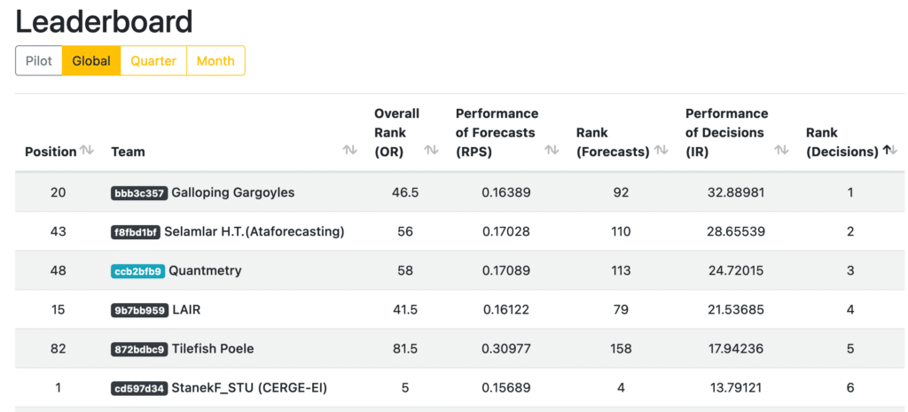
Final leaderboard of M6 competition, sorted by Rank (investment) – Link
In this post, we will delve into our winning methodology for both the forecasting and investment components of the competition. Our approach was strategic and rigorous, resulting in a solid investment decision-making process that proved successful in the competition. Join us as we share our takeaways and insights from this exhilarating competition.
Our team of Time Series data scientists at Quantmetry are thrilled to share our success in the M6 forecasting competition. After a year of hard work and dedication, we have secured the third prize in the investment component of the competition. The M6 competition challenges participants to forecast ranks for 100 financial assets and this year’s edition was particularly challenging with a live submission schedule every 4 weeks.
So what is the M6 competition?
The M forecasting competition’s 6th edition challenged more than 160 participating teams to forecast the ranks of 100 financial assets, including stocks and ETFs, in real-time. The competition required participants to submit their predicted values every month according to a specified schedule.
The competition was divided into two components: forecasting and investing. Participants had to submit exactly 12 forecasts, with each submission being required every 4 weeks. The forecasting component required the forecast of the rank probability of each financial asset, with returns in the 1st, 2nd, 3rd, 4th, or 5th quantile. The investment component involved making decisions to invest or not invest based on the forecasting probabilities estimated in the first component.
In this post, we will provide a summary of:
- Explaining the forecasting component
- Our approach for tackling the forecasting component
- Explaining investment component
- Our approach for tackling the investment component
- Takeaways
Let’s start!
(if you already know the guidelines [2] of the competition you can skip part 1 and 3 😉 )
1. Explaining the forecasting component
In this section, we will explain in detail the objective of this component.
The objective is to submit the rank probability of each of 100 assets monthly.
These 100 assets represent:
- 50 stocks from the Standard and Poor’s (S&P) 500 index
- 50 international exchange-traded funds (ETFs)

Figure 1 – A glance o some of the stocks
The 50 stocks and 50 ETFs are selected such that they are broadly representative of the global market.
The stocks represent several sectors (Financial, industrial, health care, technology, real estate, consumers good and energy) and the ETFs represents Equities, Fixed Income, commodities in different markers.
We will start by explaining step by step how to estimate the rank probability of each asset.
Step 1: For each asset, predict the stock return in 4 weeks.
Figure 2 shows the value to predict, as well the values that we can use to estimate this prediction. Noting that we can use all the historical data we want, and not exclusively those of the asset we want to predict.
The value to predict is the asset percentage change (stock return):
\[
stock\;return = \frac{Price_{J+28} – Price_J}{Price_{J}} \times 100
\]
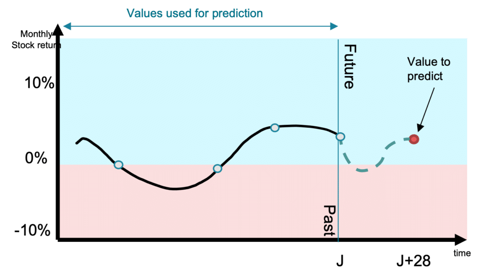
Figure 2- Timeline of features vs value to predict
Step 2: Now we have the predictions of stock return of each of the 100 assets, we will sort them from smallest to largest according to the values.
The 20 assets with the smallest values (worst performing) will be in rank 1.
- The second 20 assets with the smallest values will be in rank 2.
- The third 20 assets with the smallest values will be in rank 3.
- The fourth 20 assets with the smallest values will be in rank 4.
- The fifth 20 assets with the smallest values will be in rank 5 => the 20 assets with the largest values.
The figure 3 shows an example of how the ordering of ranks is done.
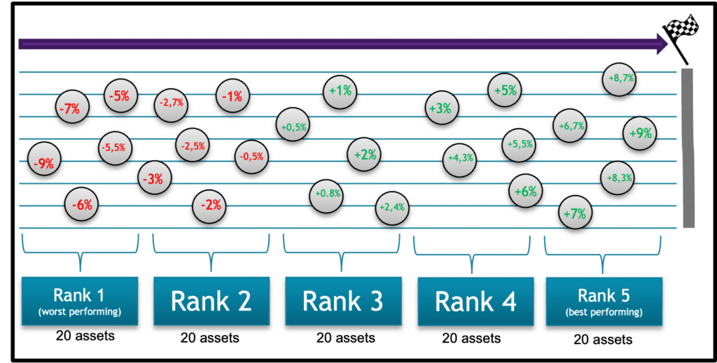
Figure 3 – The organization of assets into ranks (vertical alignment have no meaning)
Now with this, we can create the ranking table for the forecast component:
| Asset ID | Rank 1 | Rank 2 | Rank 3 | Rank 4 | Rank 5 | |
|---|---|---|---|---|---|---|
| 1 | AMAZN | 1 | 0 | 0 | 0 | 0 |
| 2 | META | 0 | 1 | 0 | 0 | 0 |
| 3 | DPZ | 0 | 1 | 0 | 0 | 0 |
| 4 | ACN | 0 | 0 | 1 | 0 | 0 |
| 5 | EWC | 0 | 0 | 0 | 1 | 0 |
| 6 | SHY | 0 | 0 | 1 | 0 | 0 |
| 7 | TLT | 1 | 0 | 0 | 0 | 0 |
| … | … | … | … | … | … | … |
| 100 | VXX | 0 | 0 | 0 | 0 | 1 |
Table 1 – Example of binary ranking of ranks
Table 1 represents the prediction of rank for each asset, we will have 20 assets predicted in the first rank, 20 in the second, etc.
This is just an example of how to create rank predictions for each asset. Of course, we are not limited to submit a binary table, instead we can submit the probability score for each asset to be in each rank. This can be achieved using different techniques that will be explained in part #2.
Measuring the performance
The forecasting performance will be measured by the Ranked Probability Score (RPS).
The RPS formula for one asset for one submission is calculated as following:
\[
RPS_{asset} = \frac{1}{5} \sum_{j=1}^{5} \left({\sum_{k=1}^{j} q_{jk} – \sum_{k=1}^{j} f_{ik}}\right)^2
\]
Where q is the true value of the rank (q is either 0 or 1) and f is the predicted probability of the rank (f is between 0 and 1).
For example, calculating RPSasset A for an asset with the following predictions.
| Asset ID | Rank 1 | Rank 2 | Rank 3 | Rank 4 | Rank 5 |
|---|---|---|---|---|---|
| Asset A | 0 | 0.2 | 0.3 | 0.4 | 0.1 |
and having as true value as Rank 4 (0,0,0,1,0) , will be :
\[
RPS_{asset A} = \frac{1}{5} \times ( (0-0)^2 + (0-0.2)^2 + (0-0.5)^2 + (1-0.9)^2 + (1-1)^2 ) = 0.06
\]
The RPS of the 100 assets is the mean of the RPS of each asset:
\[
RPS = \frac{1}{100} \sum_{i=1}^{100} RPS_i
\]
The less the RPS score, the better performing our model is.
A naïve model, predicting uniform probability for each rank of each asset will give a RPS of 0.16.
2. Approach for tackling the forecasting component
During this competition, we focused on state-of-the-art models suitable for time series forecasting task. We started by testing the Facebook Prophet model, which gave moderate results. However, we didn’t stop there and continued to explore other models. Our experimentation led us to ensemble models such as Random Forest and LGBM, which we tested extensively throughout the competition.
Two approaches were implemented:
- Regression method: For the first nine submissions, we used a machine learning approach that involved implementing several models to predict the stock return of each of the 100 assets. Each model was trained on the historical data of all the assets to predict each stock’s return at a given time. Once every model was trained, we aggregated the results and created the ranking.
This method is used for the first 9 submissions. - Classification method: we implemented a machine learning model that directly predicts the stock rank: A simple multi class classification problem. The model’s output will be the probability for each of the 5 ranks. This method is used for the rest of the submissions (last 3 submissions).
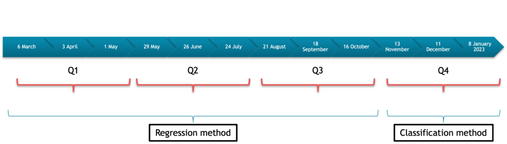
Figure 4 – Submission timeline
Features
Since we are predicting one day in the future (J + 28 days), when training we use all data prior to 28 days before the desired prediction date. (Refer to the illustrated example in figure 1)
We consider the following:
- Day J: the latest date up to which we can use historical data.
- Day J+28: the day for which we want to predict.
- Day J-X: X days prior to day J.
The following features were used:
- Calendar data (day, month, season…)
- Asset category (ETF, financial, health care, industrials, etc.)
- Historical data prior to 28 days of the prediction date (source: Yahoo [3]):
- Stock return of J relative to previous year:
- (Stock priceJ – Stock priceJ-364) / Stock priceJ-364
- Stock return of J relative to previous month:
- (Stock priceJ – Stock priceJ-28) / Stock priceJ-28
- Stock return of J relative to previous week:
- (Stock priceJ – Stock priceJ-7) / Stock priceJ-7
- Daily Exchange rates prior to 28 days of the prediction date (source: NASDAQ api [4]):
- Percentage change of exchange rate of USD to different currencies (relative to year, month, and week):
- Euro
- Canadian dollar
- Mexican pesos
- Chinese Yuan
- Japanese Yen
- Bitcoin
- Percentage change of exchange rate of USD to different currencies (relative to year, month, and week):
- Daily energy prices (gas, crude oil) prior to 28 days of the prediction date (source EIA [5]):
- Percentage change of J-28 price relative to previous year.
- Percentage change of J-28 price relative to previous month.
- Percentage change of J-28 price relative to previous week.
Other data sources were as well tested but not kept, since their availability was limit in time or frequency was very low (source: Federal Reserve Economic Data [6]):
- Daily jobs posting available since 2020 for the following countries:
- USA
- France
- Germany
- United Kingdom
- Australia
- Ireland
- US crude oil inventories available on a weekly basis
- Diverse daily financial indicators:
- ICE BofA Euro High Yield Index Effective Yield
- Moody’s Seasoned Aaa Corporate Bond Yield
- Moody’s Seasoned Baa Corporate Bond Yield
- Dow Jones Industrial Average
Regression approach
Once the features are selected, we create the features for all the training data, and we train several features combinations. In the end we kept the predictions of two models:
- Lightgbm [7]
- Random forest
For the prediction, we have two sets of 100 predictions for each model (supposed we have two models). Instead of estimating the rank probability table for each model and then calculate the mean of the two tables, we will do the following:
- For each asset, we will choose randomly one of the two predictions.
- For the randomly chosen 100 predictions of the 100 assets, we will create the rank probability table.
- Repeat step 1 and 2 ~5000 times.
Once we have 5000 ranking table, we will create the ranking prediction table to submit by simply doing the mean of the 5000 created table.
Classification approach
The same features were selected for the classification approach, but in addition to the historical stock returns features, we added the rank historical lags for each asset.
The target in this approach is not the stock return, but instead its ranking label (value from 1 to 5).
By doing so, we implemented a LGBM classifier model that directly predicts the probability of rank for each asset.
Results from both approaches
We summarize in the following table the average RPS. A reminder that a naïve model prediction 0.2 of probability for each rank for each asset will have a RPS of 0.16.
| Quarter | Approach | RPS | Rank Forecast |
|---|---|---|---|
| Q1 | Regression | 0.19509 | 130 |
| Q2 | Regression | 0.16758 | 132 |
| Q3 | Regression | 0.16401 | 128 |
| Q4 | Classification | 0.1569 | 23 |
We can see that our model was not performing well enough in the first three quarters meaning that the regression approach was not the best suited.
The classification approach gave good results on the last quarter, we were promoted up to Rank 23.
3. Explaining the investment component
We are required to submit weights for investing on each asset. It was never specified to be done according to predictions already estimated, but we decided to do so.
These weights represent the seventh column in the submitting table. They must be positive for long positions, negative for short positions and zero for no position (no investment).
Wait but what is long or short positions in finance?
Investors maintain “long” security positions in the expectation that the stock will rise in value in the future. The opposite of a “long” position is a “short” position.
A « short » position is generally the sale of a stock you do not own. Investors who sell short believe the price of the stock will decrease in value.
Reference: [8]
One interesting condition was: we were required to allocate a minimum of 25% of budget. Meaning that, we are not obliged to invest 100% of the budget but we can maintain a minimum risk of 25%.
Measuring the performance
The performance of the investment decisions is measured by means of a variant of the Information Ratio, IR, defined as the ratio of the portfolio return, to the standard deviation of the portfolio return.
We will not get into the details of this formula, but we will leave this link explaining it very well [9].
4. Approach for tackling the investment decision component
Our method was the same all along the competition. Since we were focusing on the forecasting component, we decided to minimize the risk and always invest in 25% of the budget according to this rule:
6.25% on each of the two best performing assets (the two assets with the highest probability for rank 5) = A total of 12.5 % in long position
-6.25% on each of the two worst performing assets (the two assets with the highest probability for rank 1) = A total of 12.5% in short position
We provide in the table below a summary of the ranking of our team in both components:
| Quarter | Approach | RPS | Rank Forecast | IR | Rank Investment |
|---|---|---|---|---|---|
| Q1 | Regression | 0.19509 | 130 | 7.7 | 5 |
| Q2 | Regression | 0.16758 | 132 | 5.4 | 15 |
| Q3 | Regression | 0.16401 | 128 | 8.3 | 18 |
| Q4 | Classification | 0.1569 | 23 | 3.03 | 101 |
We had a positive Information Ratio in all quarters, resulting in a sum of 24.72 in the global IR. We got the third place in the investment decision component!
| RPS | Rank Forecast | IR | Rank Investment | |
|---|---|---|---|---|
| Global | 0.17089 | 113 | 24.72 | 3 |
5. Takeaways
In the first approach, our attempt to directly predict returns using various features was unsuccessful. The machine learning models struggled to accurately forecast returns due to the high volatility of the underlying data and the influence of external factors like conflicts and crises. However, the classification approach, where we predicted rank probabilities, performed better. Surprisingly, the use of exogenous data did not improve model performance, and we found that lagged data, such as previous ranks, was more helpful in the classification task.
Overall, we are pleased to have participated in this challenging competition and maintained consistent submissions throughout. We realized the investment component was just as fascinating as the forecasting component. We gained valuable knowledge and experience during the competition, and we look forward to exploring more adaptive methods in future M competitions.
References:
[1] M6 competition
[2] M6 guidelines
[3] Yahoo Finance
[4] NASDAQ Api
[5] EIA gov
[6] Federal Reserve Bank of St Louis
[7] LGBM
[8] Long and short positions
[9] Information Ratio
La mission de l’expertise Time Series est d’exploiter le potentiel de vos séries temporelles à l’aide de solutions d’IA : analyse des données historiques, prévisions de demande, de parts de marché, de production, détection d’anomalies sur des données IoT.

Data Scientist at Quantmetry
Data scientist with a strong passion for time series and forecasting, my previous work experience involved applying my expertise to macro economies. I have since joined Quantmetry, where I collaborate with other time series experts on a variety of projects ranging from imputation to forecasting and analysis. My current role allows me to continue exploring my interests and pushing the boundaries of what's possible in this field.